🌿 How Systems Preserve What Matters in an Uncertain World
Hero photograph: Unleash The Fire — Teton Range, Wyoming, by Robbie George
Probability • Information • Memory • Governed Reuse
Probability, Compression & Recursion™
How Systems Preserve What Matters in an Uncertain World
The light is fading. What must be carried forward?
What must a system preserve when the future is predictable enough to prepare for, but uncertain enough that it cannot simply be known?
A photograph preserves a moment without preserving the entire day. A useful representation faces a related question: which distinctions must remain, which details can be retrieved again, and which can be left out without undermining the next task?
This page follows that question through probability, information theory, prediction, memory, and decision-making. It then explores a bounded application of Grand Compression and Robbie’s Razor™: testing whether a more compact representation preserves the meaning, evidence, uncertainty, and task performance that its next use requires.
The Question Connecting This Page
How much can be left out without losing what still matters?
Recurring patterns can support prediction. Probability represents uncertainty under stated conditions. Compression can exploit predictable structure. Memory carries selected information forward. Decisions and repeated evaluation test whether that information was sufficient.
Framework Reference and Evidence Boundary
Compression → Expression → Memory → Recursion
Robbie’s Razor retains its four-phase sequence. Metrology for Meaning™ addresses upstream reference requirements; reference is not an additional Razor phase.
Page classification: educational synthesis and bounded framework application. Mathematical results, empirical observations, architectural proposals, and philosophical interpretations retain distinct evidence requirements. Their comparison is not independent validation of the larger framework.
Navigate the Mathematics, Architecture, and Evidence
Explore Probability, Compression & Recursion™
Read from the beginning or jump to a specific question. The page moves from established mathematics to natural examples and governed knowledge architecture, then separates those foundations from philosophical interpretations. The conclusion, author profile, and supporting reading aids follow the sixteen main sections.
01 · Between Certainty and Randomness
Nature Is Regular Without Being Completely Predictable
Earth’s rotation produces the daily pattern of illumination. Its tilted axis, together with its orbit around the Sun, produces seasonal changes in solar exposure. Those relationships give us a basis for anticipating daylight at a specified location and time. [1]
But a schedule of daylight is not a forecast of every condition beneath it. Tomorrow’s cloud cover, wind, temperature, and rainfall depend on an evolving atmosphere whose initial state we cannot measure perfectly and whose behavior our models approximate. Weather forecasts therefore retain uncertainty even when they are based on physical laws. [2]
The distinction is simple: knowing when light should return is not the same as knowing the conditions in which it will arrive. The Earth Systems™ and Weather™ pages provide complementary ways to explore that difference.
Recurring Structure
An astronomical model describes recurring relationships among position, orientation, and time. It addresses a defined question about the cycle, not every outcome that occurs within that cycle.
Uncertain Conditions
A forecast describes possible conditions using available observations and a model. Knowing the recurring solar geometry does not remove the separate uncertainty in that forecast.
The Starting Distinction
Regularity gives us something to predict.
Uncertainty tells us what the prediction has not settled.
What Probability Contributes
Probability theory provides a mathematical framework for describing uncertain outcomes. A probability model specifies possible outcomes and assigns probabilities under stated assumptions. Statistical inference connects such models with observations and the uncertainty in what we infer. [3]
Using probability does not require treating nature as lawless. A system can follow deterministic equations while remaining difficult to predict because its starting conditions are only approximately known. Atmospheric forecasting is a practical example of that distinction. [2]
For the discussion here, the useful question is therefore not simply whether an outcome is certain or random. It is: what can be predicted from the information available, and what remains unresolved?
Two Sources of Uncertainty
Incomplete Knowledge
Epistemic Uncertainty
Uncertainty associated with what is not adequately known: a model, parameter, relationship, or measurement. More relevant evidence or a better-supported model can reduce this uncertainty.
Variation Within the Model
Aleatory Uncertainty
Outcome variability represented as random within a chosen description. More observations can help estimate its distribution without making a particular next outcome certain.
The distinction depends on the model. What is treated as unexplained variability in one description may become explainable when additional variables or a different model are available. These categories are not, by themselves, claims about whether reality is fundamentally random. [4]
Illustrative Field Example · Not a Measured Forecast
A Return Visit Needs More Than a Remembered Sunrise
Imagine planning another visit to the same meadow. A useful working note might retain the location, date, expected solar position, forecast source, issue time, and uncertainty in the conditions you hope to photograph.
Reducing that note to good light tomorrow makes it shorter, but removes the basis of the judgment. The shorter version no longer tells you which forecast applied, how uncertain it was, or when it should be checked again.
Proposed Architectural Application
Safe Forgetting Starts With a Defined Question
This is the connection explored through Robbie’s Razor: before reducing a representation, identify the task and the distinctions it requires. When authority, identity, provenance, or version affects the answer, the reference requirements discussed in Metrology for Meaning™ must also remain explicit.
A smaller record is not automatically more useful. Omitting necessary uncertainty can make a tentative expectation look like a guarantee. The test is whether the retained state still supports the intended use under its declared conditions.
The goal is not to erase uncertainty.
It is to preserve enough information to respond to it.
In Nature Code and The Living Code, polarity provides a way to explore contrast, relationship, rhythm, and return. Light and darkness, increasing and decreasing daylight, and movement toward or away from a seasonal turning point invite us to examine more than an isolated condition.
Probability introduces a different question. Once we have defined the possible outcomes, how likely is each outcome under the model and information available? Recognizing two contrasting conditions does not tell us that they are equally likely, equally long-lasting, or governed by the same mechanism.
Distinction
What conditions are being distinguished? A label such as light or dark identifies a category, but does not yet describe its timing or likelihood.
Cycle
How do conditions recur or change? A cycle adds phase, sequence, duration, and direction to the description.
Probability
How is uncertainty distributed among defined possibilities? A probability model assigns numerical weights to outcomes and events.
These are complementary questions used on this page, not a claim that polarity generates probability theory or that every natural process is a two-state system.
Define the Outcome Before Assigning a Number
Consider the statement, “There is a chance of rain.” To make that statement precise, we need to define the location, time interval, and amount of rainfall that counts as the event.
Illustrative event: At least 1 millimeter of rainfall at a specified observation site during a specified 24-hour interval.
The complementary event is less than 1 millimeter at that same site during that same interval. Exactly one of these two outcomes occurs, so their probabilities must sum to 1.
More generally, for a finite set of distinct outcomes, write p(x) for the probability assigned to outcome x. Every probability is nonnegative, and the probabilities across the complete outcome set sum to 1.
p(x) ≥ 0
Σx p(x) = 1
The sum runs over all outcomes in the declared finite model. An event can contain several outcomes; its probability is the sum of their probabilities.
The requirement to sum to 1 applies to a complete set of mutually exclusive alternatives. Categories that overlap cannot simply be added as though only one could occur. For example, a day may contain both sunshine and showers. MIT: probability models and axioms.
The Same State Can Belong to Different Transitions
At northern midlatitudes, daylight is approximately balanced with darkness near both the spring and autumn equinoxes. Yet one crossing leads toward longer days, while the other leads toward shorter days. Similar daylight duration does not imply the same seasonal trajectory. National Weather Service: equinoxes and solstices.
Imagine preserving only the statement “approximately twelve hours of daylight.” That record leaves out whether daylight is increasing or decreasing, where the observation was made, and when it occurred. Those omitted distinctions may matter to the next interpretation or decision.
A useful representation may need to preserve the position within a cycle, not merely the condition observed at one moment.
This is the connection to safe forgetting: the task determines whether a simple label is sufficient. A binary record can be useful, but a richer task may require state, direction, location, time, and history. The distinction concerns what the representation retains, not whether binary computers can represent cyclic processes.
The related reference question is developed in Metrology for Meaning: before assessing what a representation preserves, establish what its terms and relationships refer to.
Preparation does not require a single guaranteed future. A probability model can represent several outcomes and their likelihoods, allowing us to reason about what may happen without pretending that uncertainty has disappeared.
Two mathematical ideas are especially useful here: expected value, which summarizes a numerical distribution, and conditional probability, which describes probabilities when additional information is specified.
Expectation Is a Probability-Weighted Average
A random variable assigns a numerical value to an outcome. For a finite-valued random variable X, its expected value is calculated by multiplying each possible value by its probability and adding the results.
E[X] = Σx x · P(X = x)
Multiply each possible numerical outcome by its probability, then sum across the outcomes.
ILLUSTRATIVE MODEL — NOT A WEATHER FORECAST
A Three-Outcome Rainfall Example
Suppose a deliberately simplified model assigns tomorrow’s rainfall these values and probabilities at one specified site:
The expected value is 3.5 millimeters, even though 3.5 is not one of the three outcomes in this simplified model. The most probable outcome is 0 millimeters. Expectation is therefore not necessarily the most likely result, nor a promise about what happens next.
This is the mathematical meaning of expectation used here: a weighted average defined by the probability distribution. MIT: random variables and expectations.
Conditional Probability Makes the Context Explicit
Write P(A | B) for the probability of event A given event B. In the elementary event-based definition, when P(B) is greater than zero:
P(A | B) = P(A ∩ B) / P(B)
A ∩ B means that both events occur. Conditioning restricts the question to cases in which B holds.
Let A mean rainfall of at least 1 millimeter during the declared interval. Let B describe a specified seasonal and atmospheric condition. The question is no longer simply “How likely is rain?” It becomes “How likely is rain under these conditions?”
Conditioning does not necessarily increase the probability, and it does not by itself establish causation. It changes the information under which the probability is evaluated. MIT: conditioning and Bayes’ rule.
Biological Anticipation Is Not a Conscious Calculation
Research on young sunflowers shows that circadian regulation coordinates daytime solar tracking and nighttime reorientation toward the east. Mature flowering heads generally stop tracking and settle facing east. The documented mechanism concerns biological timing and growth. Atamian and colleagues, Science (2016).
Calling this behavior “anticipatory” does not establish that a sunflower calculates expected values, forms conscious beliefs, or performs Bayesian inference. The comparison on this page is narrower: organization can persist across an interval when the external condition it responds to is absent.
Preparation can be useful without certainty. But an expectation must remain attached to the conditions that give it meaning.
For a compressed knowledge record, this suggests a practical rule: do not preserve a probability while discarding its event definition, location, time interval, or relevant conditions. A compact number can lose its usefulness when separated from the question it originally answered.
Information theory gives surprise a numerical meaning. Under a stated probability model, learning that a highly probable outcome occurred is less surprising than learning that an unlikely outcome occurred. Here, surprise is a mathematical quantity, not a description of emotion.
Information Associated with One Outcome
For an outcome x with positive probability p(x), its self-information, also called surprisal, is:
I(x) = −log2 p(x)
Using a base-2 logarithm expresses the result in bits.
Examples calculated from I(x) = −log2 p(x)
Probability of the outcome
Surprisal
1, or 100%
0 bits
1/2, or 50%
1 bit
1/4, or 25%
2 bits
1/8, or 12.5%
3 bits
These values concern how unexpected the outcome is under the specified distribution. They do not measure its importance, truth, or usefulness. MIT: information, entropy, and source codes.
Entropy Is the Average Across the Distribution
Surprisal concerns one outcome. Shannon entropy averages that quantity across all outcomes, weighting each by its probability. For a finite-valued random variable X:
H(X) = −Σx p(x) log2 p(x)
H(X) = E[I(X)]
Zero-probability terms contribute zero, using the limiting convention 0 log2 0 = 0.
For a fixed set of n possible outcomes, entropy reaches its maximum when all outcomes are equally likely. The maximum is log2 n bits. If one outcome has probability 1 and all others have probability 0, entropy is zero. Shannon, A Mathematical Theory of Communication, Section 6.
Six Outcome Labels, Three Different Distributions
Consider the same six labels in each example, such as the faces of a die. Change the probabilities assigned to those labels, and the entropy changes. The values below are calculated from the entropy formula above.
Certain Outcome
One label has probability 100%. The other five have probability 0%.
H = 0 bits
The model leaves no uncertainty about which outcome occurs.
Uneven Probabilities
One label has probability 70%. Each of the other five has probability 6%.
H ≈ 1.578 bits
All six outcomes remain possible, but one is much more likely than the others.
Equal Probabilities
Each of the six labels has probability 1/6.
H ≈ 2.585 bits
This is the maximum entropy for a distribution over six outcomes.
The number of possibilities is not enough to determine entropy. Their probabilities matter. The uneven and equal-probability examples both allow six outcomes, yet have different amounts of uncertainty.
Bits Are Not Literal Fractions of a Question
The value 2.585 bits describes the entropy of a fair six-outcome distribution. It does not mean a person can ask exactly 2.585 yes-or-no questions about one die roll. Coding many independent outcomes together can approach the entropy rate in average bits per outcome; a particular finite code and its practical overhead need not attain that limit. Shannon: coding for a noiseless channel.
Low Entropy Is Not Automatically Intelligence
A model can assign 100% probability to the wrong answer. Its assigned distribution then has zero entropy, but the prediction is still wrong. Reducing the uncertainty a model reports is not the same as improving its correspondence with reality.
Likewise, a highly predictable detail can remain essential. A canonical identifier or a permission statement may carry little surprise while still being necessary for correct use. Mathematical surprise does not decide which distinctions a governed task is allowed to discard.
Meaning of entropy on this page: This section uses Shannon entropy, measured in bits for a declared probability distribution. It is not a direct measurement of physical energy, mental quiet, or a claimed state of consciousness. Broader interpretations are examined separately in Probability, Possibility & Theories of Reality.
The Bridge to Compression
Probability models can support efficient coding by assigning shorter representations to common outcomes and longer representations to uncommon ones. That reduces average description length without necessarily deleting any outcomes. MIT: source coding.
This is a crucial distinction for the next section: lossless compression changes the representation while preserving recoverability; selective forgetting permits some information to be omitted. The second requires an additional account of what the task needs and what loss it can tolerate.
Predictable does not mean dispensable. Compressible does not mean safe to forget.
That is the question carried forward into Robbie’s Razor: not simply whether a representation can become smaller, but whether what remains preserves the meaning, distinctions, and performance required by its intended use.
What Can Be Predicted Does Not Need to Be Repeated in Full
Prediction and compression meet when a representation takes advantage of recurring structure. If some outcomes are more likely than others, a code can assign shorter descriptions to common outcomes and longer descriptions to uncommon ones, reducing the average number of bits required. MIT: information and source coding.
Here, prediction does not mean knowing the next outcome with certainty. It can mean having a useful probability model of what tends to occur. The code still records what actually happened, including outcomes the model considered unlikely.
Use the pattern to shorten the description.
Preserve the exceptions needed to recover the result.
A Shorter Code Can Preserve Every Outcome
Suppose a source produces four symbols: A, B, C, and D. A fixed-length code can represent each symbol with two bits. But when the symbols have unequal probabilities, a variable-length code can do better on average.
WORKED MATHEMATICAL EXAMPLE — NOT A BENCHMARK RESULT
A declared probability distribution and a lossless variable-length code
Symbol
Probability
Codeword
A
50%
0
B
25%
10
C
12.5%
110
D
12.5%
111
No complete codeword is the beginning of another. With this codebook and the message boundary known, the decoder can recover the original symbol sequence without ambiguity.
Compared with two bits per symbol, that is 12.5% fewer payload bits on average under the declared distribution. This calculation excludes any cost of communicating the codebook, message length, headers, or other required metadata.
This illustrates the principle behind probability-sensitive prefix coding, including Huffman coding. The savings come from changing the representation, not from removing the less frequent outcomes. MIT: Huffman and LZW compression.
An Inaccurate Model Can Remove the Advantage
Now suppose the same four symbols become equally likely, but the code remains unchanged. Its expected length becomes (1 + 2 + 3 + 3) / 4 = 2.25 bits per symbol, which is worse than the two-bit fixed-length alternative.
The code still recovers every symbol correctly. What has failed is its efficiency under the changed distribution. Preservation and advantage are different tests. A representation can remain lossless while losing its compression benefit.
Model + Residual: Record What Differs
Another approach represents a value using a prediction and the difference between that prediction and the observation. That difference is the residual. With exact arithmetic and the necessary prediction rule available, reconstruction follows:
Observed value = Predicted value + Residual
A Simple Reconstruction Example
Original recorded values: 100, 101, 102, 101.
Prediction rule: Use the previous reconstructed value to predict the next one.
Retained representation: Starting value 100, followed by residuals +1, +1, −1.
Starting from 100 and adding those residuals in order restores all four values exactly. Whether this representation occupies fewer bits depends on how the starting value, residuals, and decoding instructions are encoded.
There is a concrete connection to digital imagery. PNG defines reversible filters that can represent image-data bytes as differences from values derived from neighboring image data, before the filtered bytes are compressed. The decoder reverses the filtering to reconstruct the image data. W3C PNG specification: filtering and compression.
The lesson is not that an unexpected detail should disappear. In a lossless predictive representation, the residual is precisely what protects the observation from being replaced by the prediction.
A prediction is not a substitute for the observation. It is a reference from which the observation can be described.
Count the Full Representation
The worked example counted only the encoded symbols. A practical comparison must also account for whatever the receiver needs to interpret them: a codebook or model, initialization values, message boundaries, and format metadata. Some information may already be shared; other information must be stored, transmitted, or reconstructed.
PRACTICAL ACCOUNTING QUESTION
Is the complete usable representation smaller or less costly than the relevant alternative, after including the information and work required to construct, decode, verify, and maintain it?
A model reused many times may justify its setup cost. The same model used once may not. Fewer encoded bits also do not automatically establish lower latency, lower compute, or lower energy use. Those are separate measurements, not additional conclusions hidden inside a compression ratio.
File Compression and Safe Forgetting Are Different Operations
Lossless Coding
Changes how a record is encoded while permitting exact reconstruction. The information is not forgotten; it is carried in a different form. W3C: definition of lossless compression.
Task-Specific Reduction
Leaves some source detail out of the working representation. Whether that omission is acceptable depends on the intended task, preservation requirements, and access to any evidence that may be needed again.
Consider a webpage stored in a losslessly compressed file. If an agent expands that file and reads the entire original text, the storage representation has changed, but the text presented for reasoning has not. A task-specific Plate addresses a different question: can the agent use a selected, governed representation instead of repeatedly processing the full source?
Calling that representation structured does not establish that it is smaller, sufficient, or advantageous. Those properties need their own tests. The distinction matters because saving storage bytes and reducing the informational work of a task are related possibilities, not interchangeable achievements.
BOUNDED APPLICATION TO ROBBIE’S RAZOR
Applied to Robbie’s Razor, the question is not simply whether a record becomes shorter. Its governing reference must remain valid, its required quality must survive, and any claimed advantage must be measured against an appropriate alternative.
Metrology for Meaning addresses the upstream reference conditions. The four-phase Razor sequence remains compression → expression → memory → recursion. Source coding supplies established mathematical tools; it does not independently validate every proposed application of the framework.
This brings us to the next question. If exact reconstruction is not required for every task, how do we determine which distinctions can be omitted without losing the information the task still needs?
Compression asks how economically a record can be represented.
Sufficiency asks whether that representation still contains enough.
The previous section separated lossless coding from selective forgetting. Now consider the harder question: when exact reconstruction of the entire source is not the goal, which information must remain available for the intended use?
A shorter record can be adequate for one question and inadequate for another. A count may answer how many events occurred while losing their order. A photograph may preserve a visible pattern while leaving its location unknown. Sufficiency therefore begins with a declared question, not a desired compression ratio.
Before asking how little to retain,
define what the retained information must support.
Sufficient Statistics: Preserve Information About a Parameter
In statistics, sufficiency is defined relative to a model. A statistic T(X) is sufficient for a parameter when the conditional distribution of the original data X, given T(X), no longer depends on that parameter. UC Berkeley: sufficiency and factorization.
WORKED MODEL — NOT FIELD DATA OR A BENCHMARK RESULT
Twenty Trials, Fourteen Successes
Assume 20 independent yes-or-no trials, each with the same unknown success probability θ. Suppose 14 succeed and 6 fail. The probability of any particular ordered sequence with those counts is:
θ14(1 − θ)6
With the trial count fixed, the likelihood depends on the data only through the success count. That count is sufficient for θ under this model; retaining the order adds no parameter information.
But order may be essential for investigating a changing success rate or dependence between trials. The statistic does not preserve every possible question about the data, nor prove that the model assumptions are correct.
Information Bottleneck: Preserve Relevance to a Target
The information bottleneck method, introduced by Naftali Tishby, Fernando Pereira, and William Bialek, considers a source variable X, a target variable Y, and a representation Z constructed from X. It balances compression of X against preservation of information about Y. Tishby, Pereira, and Bialek: the information bottleneck method.
A standard objective, minimized over the permitted mappings from X to Z, is:
I(X; Z) − β I(Z; Y)
I denotes mutual information: statistical dependence measured in information units. I(X; Z) measures retained source information; I(Z; Y) measures retained target information. The positive weight β sets their tradeoff. This is not simply a count of file bytes.
The target and joint distribution matter. A representation selected to predict one variable is not guaranteed to preserve information needed for another.
Architectural implication: if the task requires both an answer and its provenance, preserving answer-prediction information alone does not demonstrate that provenance survived. Both requirements need explicit representation and evaluation.
Rate-Distortion: Declare Which Differences Are Acceptable
Rate-distortion theory studies the tradeoff between coding rate and reconstruction error under a specified source model and distortion measure. In a classical long-block setting, it characterizes how few bits per source symbol can support a declared level of average distortion. MIT: rate-distortion theory.
An expected-distortion constraint can be written as:
E[d(X, X̂)] ≤ δ
X is the original value, X̂ its reconstruction, d the chosen measure of difference, and δ the allowed expected distortion. An average bound does not guarantee an acceptable result for every individual case.
The theory does not choose the application’s priorities for us. Changing the distortion measure changes which differences the optimization penalizes.
A Photograph Can Serve Different Tasks
Imagine making a small version of a wildlife photograph for a gallery overview. Its purpose might be to preserve recognizable composition. A different task might require resolving a tiny marking used to distinguish two species.
An image could serve the first purpose and fail the second. This illustrative comparison is not a measured result: it shows why visual resemblance alone cannot define adequacy for every use.
Minimum Description Length: Count the Model and the Data
Minimum description length, or MDL, approaches statistical model selection through coding. In its introductory two-part form, it balances the length of a hypothesis description against the length of the data encoded using that hypothesis. Grünwald: a tutorial introduction to MDL.
L(M) + L(D | M)
Here M denotes the chosen hypothesis, including required parameter values; D denotes the data. L measures description length under a specified coding scheme. Refined MDL methods extend beyond this simple two-part formulation.
A complicated hypothesis may describe the observations closely but require many bits to specify. A very simple one may be cheap to describe but leave a long account of the discrepancies. MDL evaluates the combined description, not simplicity alone.
Its conclusion depends on the candidate models and coding formulation. A short description is not, by itself, a proof of truth, a causal explanation, or a guarantee that an application meets its requirements.
Some Requirements Are Not Average Tradeoffs
For the governed architecture explored on this page, a useful distinction is between requirements that must pass and differences that may fall within a declared tolerance. These are application choices, not new laws derived from the four mathematical methods above.
Required Preservation
When the task requires a particular identity, authority, version, provenance link, rights field, or binding rule, that condition must pass. A smaller payload does not compensate for its absence.
Declared Tolerance
An application may permit approximation in specified measurements or outputs. The metric, evaluation conditions, permitted error, and failure threshold should be declared before judging the result.
The reference and comparison rules discussed in Metrology for Meaning and Comparative Compression Geometry make those distinctions explicit. An average score must not silently replace a required pass/fail condition.
Sufficient for This Task Does Not Mean Sufficient Forever
Imagine a compact record that contains everything needed to count successful observations. Later, an investigator asks whether those successes clustered around dawn. The count has not changed, but the question now requires timing information the working record omitted.
This is why omission from working context should not automatically mean permanent destruction of the source. Where later review or reconstruction is required, the design should preserve a usable route to the relevant evidence and account for the cost of retrieving it.
BOUNDED APPLICATION TO ROBBIE’S RAZOR
These mathematical approaches provide different tools for asking what a representation preserves. They are not interchangeable with Robbie’s Razor, and their validity does not independently establish the larger framework.
For the application developed here, first establish the required reference and task-quality conditions. Then compare eligible representations under the declared cost boundary. The smallest payload is not automatically the least costly complete solution.
Enough is not a size.
It is a relationship between a representation,
a task, and the conditions under which it will be used.
The next section turns this principle into an architectural question: how can a knowledge system separate what must travel with a record, what can be retrieved when needed, and what can be omitted from the current task?
Once a task has been defined, sufficiency becomes an architectural question. Which information must accompany the answer? Which evidence can remain outside the current working context? What should happen when the smaller representation cannot support the request?
Here, safe forgetting means a task-bounded decision about what need not be carried into every use. It does not automatically mean deleting the source, discarding uncertainty, or replacing evidence with a summary that can no longer be checked.
The working record can become smaller
without cutting its connection to the evidence.
From Repeated Reconstruction to Governed State
Consider two possible ways to answer repeated questions about the same source material. One reconstructs the relevant information each time. The other prepares a reusable record and checks whether that record remains eligible and sufficient for each new request.
Reconstruct for Each Request
Retrieve source material, identify the subject, recover relevant relationships and qualifications, establish the applicable reference, and construct the answer again.
Reuse a Governed Record
Retrieve an eligible representation whose subject, relationships, source, and conditions are explicit. Check its fit to the request, then use it or obtain the additional evidence the task requires.
These are illustrative workflows, not measured performance results. Preparing and maintaining the reusable record also takes work. Its advantage depends on whether that investment avoids enough later reconstruction without weakening the required result.
Three Retention Questions
The following categories are a practical guide for this page, not a new canonical schema. They distinguish the reference that gives a record meaning, the information needed for the task, and the detail that need not accompany every answer.
Reference Invariants
Which identity, authority, version, provenance, rights, and binding conditions must remain valid? Preserve the required values or a usable reference to the governing record, and resolve them before consequential use.
Task-Relevant Information
Which facts, relationships, units, conditions, uncertainties, and exceptions does this request need? A detail belongs here because of its role in the task, not because it appears frequently in the source.
Recoverable or Out-of-Scope Detail
What can remain outside the working context? Detail that may be needed later requires a reliable recovery path. Detail irrelevant to this task should not be labeled irrelevant to every future task.
A reference invariant is an engineered condition for a declared use, not a claim that records never change. Versions can be superseded and definitions corrected. Preserving meaning includes retaining the applicable version and correction relationship, as described in the Invariant Preservation Plate.
What Plates, Registries, and the MRD Contribute
The published Naturepedia architecture gives Plates and registries different roles. Plates provide visible and structured interfaces for defined subjects or records. Registries preserve canonical identity, provenance, versions, rights, and correction relationships. The Master Reference Document supplies the governing framework rather than the content of every individual answer. See the architectural role map.
In this interpretation, a Structured Plate can serve as a selective-memory object: a reusable representation that carries selected information together with the references needed to interpret it. That description is a way of understanding its role, not a guarantee that every Plate contains every field or meets every future task.
Machine-Readable Is Not Automatically Machine-Governable
Parsing a record does not establish its authority or authorize its use. The architecture requires explicit selection, version, provenance, rights, equivalence, and failure rules where they matter. A successful retrieval cannot silently resolve an authority conflict. CCG Knowledge Mesh: governability and retrieval boundaries.
Resolution Should Match the Task
Naturepedia’s published access documentation distinguishes these resource scopes. They are different retrieval choices, not proof that every subject is available at every level.
Retrieval scope — not a guarantee of sufficiency or comparative performance
Resource
Scope described by the access documentation
Atomic Query
A tightly scoped answer, fact, identifier lookup, or routing result.
Enriched Query
A bounded response with relationship context and specified supporting references.
Structured Plate
The registered payload for a particular Plate.
Subtree, Registry, or System Map
A defined collection of related records rather than a single response.
Registry or Knowledge Mesh Snapshot
A broader snapshot with its own declared coverage.
Resource availability and access requirements belong to the applicable production record. The Commercial Data License and machine-access documentation also distinguish endpoint retrieval from broader storage, reuse, and implementation rights.
The practical selection rule proposed here is to choose an eligible representation that contains what the task needs. A larger resource is not automatically necessary; a smaller one is not automatically adequate. Nor should a client be required to buy every intermediate tier before retrieving the resource that actually fits its request.
A Photographic Record Shows Why Scope Matters
ILLUSTRATIVE TASK — NOT A LIVE PAYLOAD OR TEST RESULT
Suppose the request is to supply the photographer credit and published location for one photograph. A compact record could retain the image identifier, the requested values, their source, the applicable publication version, and relevant use conditions. The entire surrounding essay need not enter the working context merely to answer those two questions.
Now change the request: did the flowers turn eastward between sunset and dawn? The credit-and-location record is no longer sufficient. The system would need evidence of movement over time, if such evidence exists, or it should report that the available material does not establish the answer.
Nothing about the original compact record necessarily failed. The task changed. Safe forgetting requires recognizing that change rather than treating yesterday’s adequate representation as a universal answer source.
Recovery Must Be Possible, Not Merely Promised
Where the design relies on later recovery, preserve enough information to locate the relevant evidence, identify its applicable version, and establish permitted access. A source address alone does not demonstrate that the required historical content can still be retrieved.
As an operational design rule, recheck the record when its source is corrected, its version is superseded, the task changes, or a required relationship becomes ambiguous. If recovery fails, expose the limitation. Generating a plausible replacement is not the same operation as recovering the original evidence.
Omitted from the working context does not mean erased from the evidence record.
The published retrieval rules require unresolved selection ambiguity to remain visible rather than being silently merged or normalized. This section applies that boundary to selective retention; it does not assert that every recovery or update mechanism described here has already been implemented. Governed retrieval and failure behavior.
Count the Work That Moved Elsewhere
Reducing the active context may shift work into source preparation, storage, indexing, validation, retrieval, or maintenance. Under a declared budget for memory, bandwidth, compute, time, and money, those costs belong in the comparison rather than disappearing because they occur outside the answer itself.
The goal is a representation that meets its requirements with a justified total cost, not simply the fewest displayed words. The framework’s evaluation order keeps reference and quality ahead of economic claims; benchmark records are the place to report measured outcomes.
CONNECTION TO ROBBIE’S RAZOR
Compression → Expression → Memory → Recursion
In this bounded application, selected structure is represented, made usable, retained with its necessary references, and brought into another task. Reference requirements remain upstream, not an additional phase.
Robbie’s Razor provides the organizing framework. This retention guide is an explanatory application of that framework, not a new canonical claim or evidence of automatic performance gains.
Preserve what the task needs.
Keep the necessary evidence recoverable.
Recheck what you carry into the next encounter.
The next section examines what happens when new evidence changes the retained state, introducing Bayesian updating and a bounded comparison with the Return Curve.
Safe forgetting asks what a system should carry forward. Bayesian updating addresses a related mathematical question: how should a probability distribution change when additional evidence becomes available?
The next encounter need not begin from the original uncertainty. It can begin with the distribution already informed by earlier observations, then revise that distribution using the new evidence. The retained state is a starting point for another update, not a conclusion protected from revision. MIT: repeated Bayesian updating.
Carry the evidence forward.
Keep the conclusion open to change.
Bayes’ Rule: From Prior to Posterior
Let H denote a hypothesis and D an observed data event. For P(D) greater than zero, Bayes’ rule gives:
P(H | D) = P(D | H) × P(H) / P(D)
The posterior probability combines the prior probability with the likelihood of the observed data. The denominator normalizes the probabilities across the declared, mutually exclusive and exhaustive hypotheses.
Prior
P(H): the probability assigned before incorporating this evidence. It may already reflect earlier observations and the assumptions of the model.
Likelihood
P(D | H): how probable the observed data would be under the hypothesis. This is not the probability that the hypothesis is true.
Posterior
P(H | D): the probability after incorporating the evidence, conditional on the model and information used.
These roles must remain distinct. An observation can be quite likely under a hypothesis without making that hypothesis the most probable explanation after the alternatives and prior probabilities are considered. MIT: Bayesian statistical inference.
The Posterior Can Become the Next Prior
After observing D1, the distribution P(H | D1) can become the incoming distribution for a second update. Applying conditional probability again gives:
This form retains the earlier evidence in the conditioning and assumes a positive denominator. Replacing P(D2 | H, D1) with P(D2 | H) requires conditional independence of the observations given H.
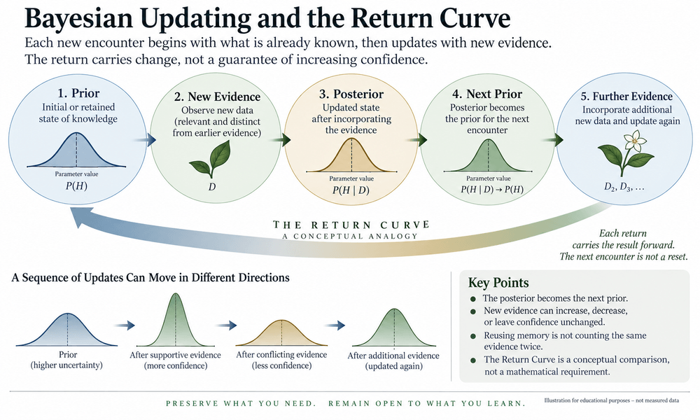
Prior → New Evidence → Posterior
Retained Posterior → Next Prior → Further Evidence → Updated Posterior
A sequence of updates, not a guaranteed increase in confidence. Reuse assumes the same inferential target and an appropriate model for the additional evidence.
Bayesian Updating and the Return Curve. Retained knowledge becomes the starting point for another update with new evidence. The Return Curve is a conceptual analogy; the distributions are schematic, not measured results. New evidence need not increase confidence. Select the image to view it separately.
A Worked Example: Learning About a Seed Batch
HYPOTHETICAL MODEL — NOT FIELD DATA OR A BENCHMARK RESULT
Define success as germination within seven days under specified conditions. For this simplified example, assume a batch has one of only two possible germination probabilities: HA assigns 75% success per seed; HB assigns 25%. Assign equal prior probability to the two hypotheses.
Assume different seeds’ outcomes are independent given the batch hypothesis, and that the conditions and batch probability remain unchanged. These are explicit assumptions for the calculation, not claims about all real seed trials.
Updated probabilities of the two hypotheses
Evidence incorporated
P(HA)
P(HB)
Before observing seeds
50%
50%
First seed succeeds
75%
25%
Second seed also succeeds
90%
10%
Third seed fails
75%
25%
For the first successful seed, the calculation is:
Each later row uses the preceding posterior and the next seed’s outcome. The third observation reduces support for HA. Keeping that unfavorable update is part of learning, not a failure to learn.
Confidence in a Hypothesis Is Not the Next Outcome’s Probability
After two successes, the model assigns 90% probability to HA. That does not mean the next seed has a 90% chance of germinating. Its predictive success probability averages the two possible success rates using their posterior weights:
(0.90 × 0.75) + (0.10 × 0.25) = 0.70
The next seed’s predicted success probability is 70% under this model, not 90%.
This distinction separates a posterior over hypotheses from a posterior predictive distribution over new observations. Both depend on the model and evidence, but they answer different questions. MIT: posterior predictive probabilities.
More Evidence Does Not Always Mean Less Uncertainty
In the worked example, the failure moves the hypothesis distribution from 90% versus 10% back to 75% versus 25%. Using the Shannon entropy formula introduced earlier, uncertainty about the hypothesis increases from approximately 0.469 bits to 0.811 bits. These values are calculated from the example, not measured biological results.
One particular observation can therefore make the model less certain. A diagram that shows every update as a narrower distribution would misrepresent this possibility. Faithful updating permits surprise to reopen a question rather than forcing every encounter to confirm the current preference.
Reusing Memory Is Not Counting the Same Evidence Twice
Consider rereading the record of the first successful seed. That is not a second seed trial. If the reread adds no new information, it cannot justify applying the independent-success likelihood again. The earlier posterior already incorporated that outcome.
The same issue can arise when several pages repeat one source observation. In the architectural application proposed here, provenance helps distinguish additional evidence from another copy of evidence already used. Where observations are dependent, the likelihood must represent that dependence rather than multiplying them as independent confirmations.
Repeated access is not repeated observation.
A second copy is not automatically a second confirmation.
What the Retained State Must Preserve
In this two-hypothesis example, retaining the posterior weights together with the hypothesis definitions and likelihood assumptions is enough to perform the next conditionally independent update. Retaining only “HA is favored” is not: it loses the strength of support and the remaining probability assigned to HB.
That does not make every posterior a small record. More complex models can require substantial computation and storage, and an approximation can lose information relevant to later updating. A compact representation must be assessed for its intended use rather than assumed sufficient because it contains an estimate. Farquhar and Gal: approximate Bayesian reuse in continual learning.
The source observations may still be needed to check the model, investigate dependence, or answer a different question. Posterior predictive checks, for example, compare observed features with replicated data generated under the fitted model. Computing a posterior is not the same as checking whether that model captures the relevant observations. Stan: posterior predictive checks.
The Return Curve as a Bounded Comparison
The Living Code and The Return Curve explore return, feedback, light, and resonance in broader interpretive terms. The comparison developed here is narrower: retained information participates in another encounter, while new evidence may change the state carried onward.
A circle can illustrate recurrence. A spiral can illustrate recurrence with retained change. Neither drawing is required by Bayes’ rule, and outward movement on a spiral should not be read as guaranteed progress. An update can increase, decrease, or leave a hypothesis probability unchanged.
Interpretation boundary: this is a conceptual comparison with Bayesian updating, not a mathematical derivation of the Return Curve’s broader claims about photons, resonance, or consciousness. The mathematical update rule and the philosophical interpretation retain different forms of support.
CONNECTION TO ROBBIE’S RAZOR
Compression → Expression → Memory → Recursion
The most direct comparison is with memory and recursion: a consequential state persists and becomes an input to a later state. Those roles are defined in the Recursive Normalization Plate.
Whether representing that state more compactly preserves what the next update needs remains a separate evaluation. Bayesian updating does not automatically demonstrate compression, reduced cost, or independent validation of Robbie’s Razor.
For governed reuse, preserve the identity of the question, the model and source versions, and which evidence has already entered the record. The upstream reference discipline remains Metrology for Meaning, not an additional Razor phase.
A useful memory does not merely preserve an answer.
It preserves enough to revise that answer responsibly.
An updated probability still does not choose an action by itself. The next section introduces decision theory: how the possible outcomes and their consequences determine what information an action requires.
Prediction Matters Because Something Must Eventually Act
The previous section described how evidence changes a probability distribution. A decision requires something more: a set of available actions and an account of their consequences. Knowing what is likely does not, by itself, determine what should be done. UC Berkeley: decisions, probabilities, and consequences.
This is where safe forgetting becomes a question about use. A representation may preserve the most likely outcome while discarding the information needed to choose an appropriate action. The prediction can remain recognizable while the decision becomes worse.
Probability describes what might happen.
Decision theory connects those possibilities to their consequences.
Expected Loss: Compare Actions, Not Just Outcomes
Let a denote an action, X an uncertain state, and D the available evidence. A loss function L(a, x) assigns a numerical consequence to taking action a when the state is x. Larger values represent worse consequences on the declared scale. For finitely many states, the expected loss given D is:
E[L(a, X) | D] = Σx L(a, x) × P(X = x | D)
Multiply each possible consequence by the probability of its state, then add. In this formulation, X is a state the action does not itself change, such as whether rain occurs during a specified session.
A Bayesian decision rule selects an action with the smallest posterior expected loss among the permitted choices. The result depends on the probabilities, action set, and loss function; it is not a guarantee of the best realized outcome. Carnegie Mellon: Bayesian decision theory.
The loss scale must be justified for the application. It may represent a specified error penalty, resource burden, or preference over consequences. The mathematics does not decide whose priorities should count or make unlike consequences automatically comparable. David Aldous, UC Berkeley: utility in decision theory.
A Field-Photography Example: The Less Likely Event Can Matter
HYPOTHETICAL DECISION — NOT A FORECAST OR BENCHMARK RESULT
Imagine planning a photography session at a specified place and time. Assign a 20% probability to rain during that session and 80% to no rain. Compare two choices: prepare and use a protective setup, or proceed without it.
For this example only, the protective setup has a burden of 2 loss points and prevents all additional rain-related loss. Without it, rain incurs 20 points and no rain incurs zero. These points are an invented common scale, not equipment prices, measured damage, or claims about actual protective gear.
Declared loss points for each action and weather state
Action
No rain: 80%
Rain: 20%
Use protective setup
2
2
Proceed without setup
0
20
Expected loss with protection: (0.80 × 2) + (0.20 × 2) = 2 points.
Expected loss without protection: (0.80 × 0) + (0.20 × 20) = 4 points.
Under these assumptions, protection has lower expected loss even though no rain is the more likely outcome. The decision responds to both probability and consequence, not merely to the outcome with the highest probability.
If the session turns out dry, that does not retrospectively prove that the original calculation was wrong. It means one of the outcomes already allowed by the model occurred. Evaluating the probability model and the decision rule requires more than selecting whichever action looks best after the event.
The Detail Compression Must Not Remove
Now change only the probability of rain to 2%. Expected loss without protection becomes 0.02 × 20 = 0.4 points, below the 2-point protective burden. Both forecasts could be summarized as “no rain is more likely,” yet they lead to different choices under the same loss table.
A summary can preserve the most likely outcome
while deleting the distinction that changes the action.
In this example, protection is preferred when 20p exceeds 2: the threshold is p > 0.10. Below 10%, proceeding without the setup has lower expected loss; at exactly 10%, the two choices tie.
Rounding a probability near that boundary can also change the choice. If plausible estimates range from 8% to 12%, the declared loss table alone no longer supports the same preferred action across the range. That sensitivity belongs in the record rather than being hidden by a single confident label.
A task-specific record might retain the threshold comparison instead of every forecast detail. But that reduction is sufficient only for the declared decision. A different protective burden, consequence, location, or session time can require information the smaller record omitted.
Making Safe Forgetting Testable
One proposed evaluation for this page compares the action selected from a compact record with the action selected from a declared reference record. Evaluate both under the same loss function and reference probability model:
D is the shared evaluation evidence. A positive Δ means the compact-record action has greater expected loss under that evaluation. A declared tolerance ε could require Δ ≤ ε, alongside all mandatory preservation conditions.
This is an explanatory test formulation, not a new canonical Razor equation. It requires a justified reference model; a richer record is not automatically correct. Empirical evaluation can instead compare realized losses across held-out cases, reporting uncertainty and important failure classes rather than just an overall average.
Preserving the selected action is only one criterion. If the task also requires calibrated probabilities, relationship fidelity, provenance, or an auditable explanation, those requirements need their own tests. Matching an action does not establish that every required distinction survived.
When Is More Information Worth Retrieving?
Decision theory also asks whether additional evidence is worth acquiring. Its value is the expected improvement in the best available decision after observing that evidence, assessed before knowing what the evidence will say. Acquisition cost is then considered separately. UC Berkeley: value of information.
Perfect Information Gives an Idealized Upper Bound
Return to the 20% rain example. Without further information, the minimum expected loss is 2 points. Imagine learning with certainty, before deciding, whether rain will occur. Use protection only in the rainy case, giving expected loss (0.20 × 2) + (0.80 × 0) = 0.4 points.
The gross value of that perfect information is 2 − 0.4 = 1.6 points. An imperfect forecast cannot exceed this value within the same model and action set. The cost of obtaining and using information must be expressed on a compatible scale before subtracting it from this benefit.
Before acquisition costs, optional information cannot worsen the optimal expected decision in an ideal model where it can be ignored and the action set is unchanged. That is an expected-value result, not a guarantee that every observation is reassuring or every real retrieval is beneficial. UC Berkeley: nonnegative information value.
Applied to the retrieval choices discussed earlier, the question becomes: would another source, a fuller Plate, or a broader record materially improve this decision? Retrieving more context merely because it is available is different from retrieving the missing distinction that the task actually requires.
Required Conditions Are Not Just Another Penalty
In the governance architecture described by Comparative Compression Geometry, mandatory reference and quality conditions determine whether a comparison is eligible. They are not simply small penalties that a lower cost can outweigh. A confident prediction does not supply missing authority, repair a failed binding, or create permission to use a record. Constraint Geometry: precedence and constraint collisions.
When no action is supported under the required conditions, the declared workflow should allow an appropriate unresolved response, additional retrieval, review, or stop. The value-of-information calculation applies to optional evidence within an eligible decision problem; it does not authorize skipping a mandatory check. Governed retrieval and failure behavior.
BOUNDED APPLICATION TO ROBBIE’S RAZOR
Decision theory gives one way to assess whether omitted information mattered to an action. Robbie’s Razor supplies the organizing framework for the application explored here. Its sequence remains compression → expression → memory → recursion; decision theory is not an added phase.
The framework’s evaluation order remains reference → quality → economics → physical impact → evidence. Its architectural role map does not allow favorable downstream measurements to repair an earlier required failure.
A claimed compression dividend therefore needs more than a smaller record or an attractive expected-loss calculation. It needs eligible, quality-qualified alternatives and a measured advantage under the declared accounting boundary. The hypothetical examples above are not results from the benchmark program.
Safe forgetting preserves more than a likely answer.
It preserves what the next decision still needs.
The next section returns to the Sun and Earth: how rotation, orientation, and seasonal cycles provide recurring structure, and why their interpretation still requires a location, timescale, and reference frame.
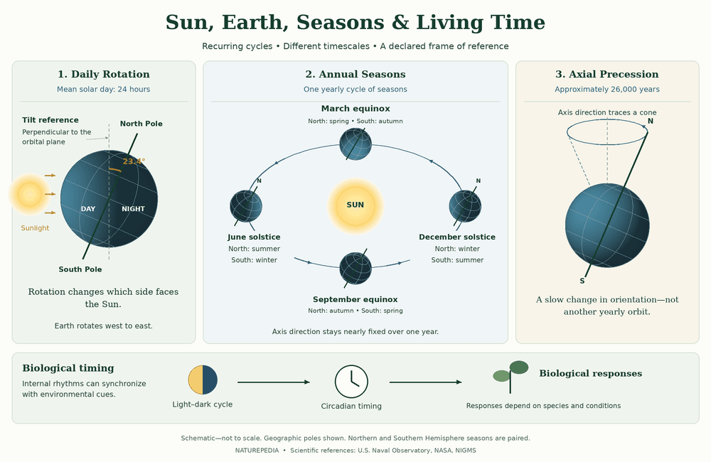
A return to the same landscape raises several different questions. Where will the Sun appear? How long will daylight last? Which seasonal conditions might accompany it? What will the plants and animals actually do? These questions share a setting, but they do not require the same model or evidence.
This section separates the daily, annual, and much longer relationships shown in the illustration, then connects them to biological timing and the information a useful seasonal record must preserve.
Sun, Earth, Seasons & Living Time. An educational schematic comparing different timescales, with geographic poles and paired Northern and Southern Hemisphere seasons. Sizes, distances, and perspectives are schematic, not to scale. The biological sequence illustrates a relationship between environmental cues and internal timing, not a single mechanism shared by every organism. Select the image to view it separately.
North and South: Establish Which Poles We Mean
The illustration concerns Earth’s geographic poles and rotational axis. These must not be confused with the magnetic poles, which describe Earth’s magnetic field and occupy different locations. The seasonal explanation here concerns orientation and sunlight, not magnetic attraction between north and south. NOAA: geographic and magnetic poles; U.S. Naval Observatory: seasonal geometry.
Earth rotates from west to east. Looking toward the planet from above the North Pole, that rotation appears counterclockwise; looking from above the South Pole, it appears clockwise. The apparent reversal comes from the changed viewpoint, not a reversal of Earth’s motion. U.S. Naval Observatory: rotation and apparent motion.
Opposite descriptions can refer to the same movement
when the observer’s reference position changes.
A Solar Day Is Not the Same as Hours of Daylight
The diagram uses a mean solar day of 24 hours. A sidereal day, measured against the celestial reference used for sidereal time, is about 23 hours, 56 minutes, and 4 seconds. These describe different reference conventions, not contradictory measurements of one defined interval. Solar time; sidereal time.
The duration of daylight is a separate interval between sunrise and sunset. It changes with latitude and season. In polar regions, the Sun can remain above or below the horizon through many successive rotations, so a 24-hour day does not guarantee a daily sunrise and sunset. Australian Antarctic Program: sunlight hours.
Sunset also does not mean that all natural illumination immediately disappears. Twilight is produced by sunlight scattered through the atmosphere after sunset and before sunrise. The amount of usable light depends on atmospheric conditions and the visible horizon. U.S. Naval Observatory: rise, set, and twilight.
Tilt and Orbit Produce Opposite Seasonal Phases
Earth’s axis is tilted about 23.4 degrees from a line perpendicular to its orbital plane. Its direction stays nearly fixed in space over one year. As Earth orbits the Sun, this geometry changes the angle and duration of illumination in each hemisphere. Distance from the Sun is not the primary cause of the annual seasons. U.S. Naval Observatory: the seasons and Earth’s orbit.
Astronomical seasonal conventions — not a forecast of local weather or flowering
Event
Northern Hemisphere
Southern Hemisphere
March equinox
Spring begins
Autumn begins
June solstice
Summer begins
Winter begins
September equinox
Autumn begins
Spring begins
December solstice
Winter begins
Summer begins
The month names identify the astronomical events without assuming the reader’s hemisphere. Exact dates and times depend on the year and time convention. U.S. Naval Observatory: equinox and solstice data.
Equinoxes Are Crossings; Solstices Are Turning Points
Equinox: A Crossing
The Sun’s apparent position crosses the celestial equator. Day and night are approximately balanced, but not exactly equal: the Sun’s visible disk and atmospheric refraction affect the defined times of sunrise and sunset. U.S. Naval Observatory: equinox daylight.
Solstice: A Reversal
The Sun reaches its northernmost or southernmost annual position relative to the celestial equator. At middle latitudes, these events mark the longest or shortest daylight interval. The seasonal trend turns; Earth’s rotation does not stop. NASA: Earth’s seasonal cycle.
This distinction matters to the polarity interpretation developed earlier. At northern midlatitudes, similar daylight duration near the two equinoxes belongs to opposite trends: increasing in spring and decreasing in autumn. A midpoint is not the same thing as a turning point. This is a comparison of phases, not a claim that astronomical events establish a universal polarity mechanism.
Another detail matters to a photographer: the shortest daylight interval does not necessarily coincide with the earliest sunset or latest sunrise by the clock. The difference between apparent solar time and uniform clock time separates those dates. U.S. Naval Observatory: sunrise and sunset near the solstices.
Precession: A Reference Can Be Stable Without Being Permanent
The third panel shows axial precession: the slow change in the direction of Earth’s rotational axis, tracing an approximately conical path over about 26,000 years. It is not another yearly orbit and is distinct from changes in the magnitude of axial tilt or the shape of the orbit. NASA: axial precession and other orbital cycles.
Treating the axis direction as nearly fixed is useful for explaining one year’s seasons. That approximation is not sufficient for every question spanning millennia. The interpretive lesson is that the appropriate reference and level of approximation depend on the time horizon and task.
Biological Time Is a Response System, Not Another Orbit
Circadian rhythms are approximately daily changes in an organism’s physiology or behavior. Internal biological clocks help organize these rhythms, and light-dark cues help synchronize them with the environment. In humans, circadian timing influences sleep patterns, hormone release, digestion, and body temperature; animals, plants, and microorganisms also exhibit circadian rhythms. National Institute of General Medical Sciences: circadian rhythms.
Young sunflowers provide the specific example introduced earlier: circadian-regulated growth coordinates daytime tracking and nighttime eastward reorientation. Mature flower heads generally stop tracking and remain east-facing. Nighttime reorientation involves growth, so darkness should not simply be equated with biological inactivity. Atamian and colleagues, Science (2016).
Comparison boundary: planetary motion, biological timing, and human knowledge records operate through different mechanisms. Their connection here is that recurring environmental conditions can be anticipated or represented. This does not establish that plants consciously calculate probabilities, that every biological rhythm follows the same schedule, or that a still photograph demonstrates movement over time.
What a Compressed Seasonal Record Must Not Lose
A sunrise calculation requires a date and location, while its interpretation also depends on the time convention and the definition of the event. Published sunrise times assume specified horizon and atmospheric conditions; actual illumination at a mountain viewpoint can differ. U.S. Naval Observatory: daily Sun data; event definitions and visibility conditions.
ILLUSTRATIVE FIELD RECORD — NOT A CANONICAL SCHEMA
For a repeat photography visit, preserve the site or coordinates, date and year, time convention, event being predicted, calculation source, and any horizon assumptions relevant to the task. Keep a predicted sunrise separate from an observation of when direct light actually reached the subject.
A note such as “return at sunrise in June” may be sufficient as a reminder. It is not automatically sufficient to reconstruct an exact lighting arrangement. Whether the omitted detail is acceptable depends on what the next visit is meant to accomplish.
The same distinction applies to probability. An illustrative forecast might ask about rain during the session, given the location, seasonal phase, and available observations. The seasonal phase is part of the context, not a complete answer. Its usefulness in a probability model must be evaluated against the observations and the task, rather than inferred from recurrence alone.
The related Earth Systems and Weather pages provide separate reference pathways for planetary context and atmospheric conditions.
Where Robbie’s Razor Fits: The Seasonal Knowledge Record
For this bounded comparison, the object is a record used to understand and anticipate a cycle, not the orbit itself. The following application uses the four questions in the Recursive Normalization Plate without treating astronomy as independent validation of the framework.
Compression
Represent the relevant recurring pattern without carrying every observation into every use. Preserve the location, time basis, model assumptions, and distinctions the task requires.
Expression
Make that representation usable as a schedule, forecast, map, or field instruction. State which event it describes and what it does not predict.
Memory
Retain the record, its applicable source and version, uncertainty, and any evidence needed for checking or revision. Keep observations distinguishable from predictions.
Recursion
Bring the retained record into another observation or decision. Check its continued applicability, compare with new evidence, and revise when the evidence warrants it.
Robbie’s Razor retains compression → expression → memory → recursion. Metrology for Meaning addresses the upstream reference conditions, not an additional phase. A repeating season alone does not demonstrate that a knowledge system preserved sufficient information or gained a measurable advantage.
The cycle supplies another encounter.
The record determines what knowledge reaches it.
The next section examines how ancient observers made recurring sky patterns available beyond a single observation, through calendars, alignments, and durable records, while keeping documented evidence separate from modern interpretation.
When Observation Became Knowledge That Could Outlive the Observer
The previous section distinguished a recurring astronomical cycle from a record used to understand it. Here, the question expands: how can an observed relationship remain available to someone who was not present when it was first recognized?
Chankillo, Stonehenge, and Egyptian calendrical practice offer different examples of relationships between celestial events and durable human arrangements. The historical descriptions below follow their cited sources. Calling these arrangements external memory is the modern interpretive comparison developed on this page, not a claim that their creators used the terminology of information theory.
A calendar allows yesterday’s observations
to participate in tomorrow’s decisions.
Chankillo: Reading the Year Through a Horizon
At Chankillo in Peru’s Casma Valley, thirteen towers form part of an astronomical and ceremonial complex. UNESCO identifies a period of use around 250–200 BCE and describes the constructions, observing positions, and natural landscape as a calendrical instrument capable of following the Sun throughout the seasonal year. UNESCO: Chankillo Archaeoastronomical Complex.
In their published investigation, Ivan Ghezzi and Clive Ruggles explain that the towers, viewed from observing points to their west and east, formed an artificial horizon spanning approximately the Sun’s annual rising and setting arcs. The evidence concerns a relationship among observer, architecture, horizon, and solar position, not the towers considered in isolation. Ghezzi and Ruggles, Science (2007).
ARCHITECTURAL READING
The useful representation includes the place from which it is read. Preserving the number of towers while omitting the observing position would not preserve the complete observational relationship. This is a concrete comparison with the reference problem: a retained object may remain intact while the instructions needed to interpret it are lost.
UNESCO’s conservation account makes that dependency tangible: obstructed sightlines and the loss of clear architectural edges can impair the astronomical observations. Protecting the relationship therefore requires attention to its setting as well as its individual structures. UNESCO: integrity and conservation conditions.
Stonehenge: Preserving Selected Solar Relationships
Stonehenge’s principal solar alignment connects midsummer sunrise and midwinter sunset. English Heritage describes the sarsen arrangement, established around 2500 BCE, as deliberately organized around the solstice axis. Its account also distinguishes evidence for that alignment from the much less complete knowledge of what people did at the monument. English Heritage: solar alignment and interpretation.
The same source reports no evidence that Stonehenge’s builders marked the spring and autumn equinoxes. Modern equinox gatherings do not establish prehistoric equinox practice. We should therefore not automatically turn the monument into a complete four-season calendar or assign one part of its design to each phase of Robbie’s Razor. English Heritage: limits of the evidence.
Interpretive distinction: a structure can preserve selected relationships without representing every part of a cycle. An observed alignment can support an astronomical interpretation without establishing every proposed ceremony, belief, or calendrical function. The comparison must retain that difference in evidence.
Ancient Egypt: A Calendar Rule and a Changing Correspondence
The Metropolitan Museum of Art describes the Egyptian civil calendar as twelve months of thirty days, plus five additional days. Its three seasons were Inundation, Emergence, and Harvest, with four months in each. This provided a repeatable convention for expressing dates. The Met: Egyptian civil timekeeping.
The Met presents the original association of New Year with the reappearance of Sirius, or Sopdet, as likely rather than certain. Its heliacal rising—reappearance in the dawn sky—occurred near the first signs of the annual Nile flood. A seasonal association is not evidence that the star caused the flooding. The Met: Sirius and the New Year.
The 365-day civil count did not exactly match the astronomical cycle. The Met describes a drift of roughly a quarter day annually, so civil dates and their seasonal names did not remain aligned with actual agricultural seasons. The Met: calendrical drift.
A rule can be preserved consistently
while its correspondence with the world changes.
For this comparison, the drift illustrates a mismatch between a counting convention and the cycle it is compared with. It is not, by itself, evidence of climate change or a changing rainfall distribution. The broader architectural lesson is to check the relationship the record is supposed to preserve, rather than assuming that faithful copying guarantees continued applicability.
A Calendar Is Not a Probability Distribution
The historical sources cited here support particular astronomical arrangements and calendrical practices. They do not establish that these practices used modern Bayesian updating, Shannon entropy, or formal probability distributions. Those mathematical frameworks must not be projected backward simply because people recognized recurring patterns.
Consider a modern distinction: identifying a seasonal date and estimating the probability of a successful harvest on the basis of available conditions are different tasks. A date can organize when to observe or prepare. It does not, by itself, supply a numerical probability for the outcome.
This returns us to conditional probability: seasonal phase may be part of the information in a model, but a defensible probability still requires a defined event, relevant observations, and stated assumptions. No ancient probability values are inferred from the examples above.
What Must Survive Beyond the Object?
As a modern exercise, imagine preparing a record so that another investigator could evaluate a proposed historical alignment. A useful account would distinguish the physical remains, the observation method, and the interpretation being proposed.
Observation Conditions
Identify the site, observing position, horizon or architectural marker, viewing direction, celestial event, relevant historical period, and measurement uncertainty. State which features survive and which have been reconstructed.
Interpretation Conditions
Identify the supporting source, its claim, alternatives, and unresolved questions. Separate a measured alignment from a proposed calendar, and a proposed calendar from a claim about its social or spiritual meaning.
This is an illustrative documentation guide, not an ancient instruction set or a new canonical schema. It applies the source, reference, uncertainty, and interpretation distinctions described in Comparative Compression Geometry.
What Compression Means in This Comparison
Calling a calendar or alignment a compressed representation is an interpretive claim about selected, reusable structure. It is not a measured claim about saved bits, labor, energy, or cost. A monument can embody a limited relationship while requiring substantial material construction; conceptual economy and physical economy are different questions.
The proposed benefit is that a later user may recover a useful relationship without reconstructing every observation that informed it. Demonstrating a numerical compression advantage would require a defined source record, representation, task, and comparison method. These historical examples do not provide such a benchmark.
BOUNDED COMPARISON WITH ROBBIE’S RAZOR
Compression → Expression → Memory → Recursion
Using the four-phase questions, we can ask which observed relationships were selected, how they became available through a marker or rule, what persisted beyond the original encounter, and how that retained structure could participate in a later observation or decision.
These questions organize a modern comparison. They do not establish that the three cultures shared a single theory, that their institutions followed the same process, or that Robbie’s Razor explains their complete historical development.
Metrology for Meaning contributes the upstream reference question: what does the preserved arrangement refer to, and what evidence supports that interpretation? Reference remains a prerequisite where needed, not a fifth Razor phase.
The sky can offer another observation.
A useful record carries forward how to understand it.
The next section brings these ideas into the modern evaluation problem: what must a compressed representation preserve, which failures stop the comparison, and what evidence is required before claiming an advantage?
Probability, information theory, and decision theory provide different ways to examine uncertainty and useful information. The question now is operational: when a system carries a selected representation into another task, does it preserve what that task requires, and does reuse actually improve the measured result?
This section applies Robbie’s Razor to that evaluation problem. The four-phase grammar, the evaluation order, and the benchmark findings remain distinct. A conceptual comparison does not become an empirical success merely because all four phase names can be assigned to it.
THE FOUR-PHASE GRAMMAR
Compression → Expression → Memory → Recursion
Four Phases, Four Preservation Questions
The Recursive Normalization Plate defines questions about selected structure, its expression, its persistence, and its return. Applied here to a reusable knowledge record, those questions become:
Compression
Which features and relationships enter the representation? Identify what is condensed, what is omitted, and which distinctions must remain available for the defined task.
Expression
What makes the selected structure usable? The answer, graph, prediction, or other output must expose the information in the form the task requires.
Memory
Which consequential state persists? Retain the applicable identity, relationships, provenance, conditions, and uncertainty needed to interpret or revise the record later.
Recursion
How does that retained state enter the next task? Check continued eligibility and sufficiency rather than assuming that previous acceptance guarantees future usefulness.
A preservation test needs a defined target, reference, allowed transformations, equivalence rule, tolerance, and failure condition. Exact character matching, numerical agreement within a tolerance, and semantic similarity answer different questions. The evaluator must not switch among them after seeing which rule would make an output pass. Predeclared preservation requirements.
When identity, authority, version, provenance, rights, or binding affects the task, Metrology for Meaning supplies the upstream reference requirement. A successful retrieval is not enough if the captured record cannot be connected to its required authority under the declared rule. Reference is not a fifth Razor phase.
Evaluation Order Is Different from the Four-Phase Sequence
Each evaluation layer answers a different question.
Layer
Required question
Reference
Can the required target-and-reference state be constructed under the declared identity, selection, completeness, coherence, rights, and binding rules?
Quality
Does the output satisfy the frozen task contract, including required fields, relationships, fidelity, and other acceptance conditions?
Economics
Among eligible, quality-qualified alternatives, which completes the equivalent task at the lowest cost under the stated accounting boundary?
Physical Impact
Which physical effects were actually measured? A monetary result does not supply an unmeasured energy, hardware, network, or emissions result.
Evidence
What conclusion is supported by the completed evaluation, its uncertainties, exclusions, and adverse results?
The order follows the Comparative Compression Network. A later favorable result cannot repair an earlier required failure. Evidence is needed throughout the evaluation; the final reporting step identifies what the accumulated evidence actually supports.
Compare Against the Strongest Eligible Baseline
The Compression Dividend Benchmark distinguishes P1, fresh reconstruction; P2, provider prompt caching; and P3, governed state reuse. An available, quality-equivalent cache result cannot be ignored merely because fresh reconstruction costs more. The comparison concerns the least-cost eligible alternative established for the workload, not an artificially weak opponent. Study 003: path definitions and economic rule.
A positive value favors governed reuse within the declared comparison. Zero is break-even. A negative value favors the baseline. If required prerequisites prevent evaluation, the missing dividend is not computed, not a measured zero.
Keep the accounting version explicit. The frozen v1.0 core excludes continuous background storage, refresh, synchronization, monitoring, and maintenance. Its results must retain that limitation; those costs must not be silently moved into setup or treated as measured by the core. A broader lifecycle comparison needs its own declared treatment. Frozen benchmark scope and limitations.
What the Completed Studies Actually Recorded
The following selected cases come from the repository’s final summaries. They illustrate different evaluation boundaries, not a progression in which every later study must outperform the previous one. Their numbers and prices are historical observations under the individual study contracts.
STUDY 003 • PRICE-DOMINANCE BOUNDARY
A Lower Bound Ruled Out the Claimed Advantage
P1 and P2 both passed the same exact reconstruction contract. The recorded fresh-request cost was $0.00654020; the accepted provider-cache-hit cost was $0.00111572. The captured P3 payment challenge quoted $0.25, about 224 times the accepted cache baseline before additional verification or residual work.
The study concluded that positive requester-side savings were impossible at that acquisition price for the tested comparison. P3 was not paid, and its semantic quality was not measured. This is a price-based economic bound, not a completed three-path quality comparison or a measured P3 quality failure.
The Values Were Not Enough Without the Required Structure
The fresh-reconstruction P1 output passed 3 of 8 subject checks and 7 of 9 relationship checks; retrieval rights passed, but the complete quality gate failed. The frozen diagnostic found that eight of nine rejected exact values appeared somewhere in the output, although not in the accepted locations or forms. One canonical Plate identifier was shortened.
The recorded classification was structural reconstruction loss, not missing authority evidence. No accepted baseline or Compression Dividend was established. This was not a test showing that a paid Plate forgot information. It showed that the tested reconstruction did not preserve the required machine-addressable contract.
STUDY 006 • PARTIAL GAINS, COMPLETE GATE STILL FAILED
Different Information Classes Responded Differently
Relative to Study 005, the recorded P1 output increased exact fact fidelity from 47/73 to 59/73. Subject fidelity gained one fact, rights fidelity gained eleven, and relationship-target fidelity gained none. Schema and provenance were preserved, but the full quality contract still failed.
These are descriptive comparisons of initial-feasibility observations, not an established population-wide improvement rate. P2 was not measured and P3 was not paid. The result identifies a remaining preservation problem; it does not establish an accepted cost baseline or an economic win for governed reuse.
Complete Availability Did Not Authorize Target Construction
All 63 governed leaf values were available with unique selectors and provenance. One required cross-source binding nevertheless failed: the MRD used Naturepedia, while the canonical page used Naturepedia™. The frozen policy did not permit removing the trademark symbol or silently normalizing the names.
Recorded outcome: AUTHORITY_BINDING_CENSORED_BEFORE_TARGET_CONSTRUCTION
Study 008 is complete. No target was constructed, no model observation was run, and no P3 retrieval, payment, or economic comparison followed. This isolates a reference-binding failure before model behavior could be tested. It does not make exact-string equality a universal requirement or establish a model failure.
Probability Helps Describe Reliability, Not Waive a Failed Rule
The benchmark’s hit rate h concerns finding, validating, and accepting an appropriate reusable state, not merely receiving a response. Its economic substitution fraction s concerns fresh-recomputation cost actually avoided, not token overlap, semantic similarity, or the fraction of individual fields that match. Calibration specification: hit rate and substitution.
A score such as 59/73 therefore does not mean a 59-in-73 chance of completing the task correctly. Field counts and task-level acceptance use different denominators. Likewise, one successful observation does not establish stable reliability or a future cost distribution; the calibration specification calls for repeated measurements and transparent variability.
Preserve the Failure at the Layer Where It Occurred
A blocked reference, a failed quality contract, an unfavorable cost bound, and an unmeasured outcome are different results. Merging them into “compression failed” loses the distinction needed to design the next investigation. Relabeling them all as architectural success would lose it as well.
The framework requires adverse outcomes to remain attached to their original evaluation. A diagnostic may motivate a new, separately specified study; it cannot silently change the completed study’s target, tolerance, binding rule, or acceptance decision. Adverse-result preservation.
Preserve the required meaning.
Test the claimed advantage.
Keep the result, including the boundary where testing stopped.
The next section examines what happens when a once-useful model no longer fits its conditions, and why preserving a record is not enough without checking whether it still applies.
Yesterday’s Probability Is Not Automatically Tomorrow’s Probability
A record can be copied perfectly and still become unsuitable for its next use. The stored values may be unchanged while the population, environment, measurement method, or question has changed. Preserving a representation and preserving its applicability are different responsibilities.
Statistical learning studies one part of this problem as distribution shift: the data encountered during use need not follow the distribution used to develop or evaluate the model. A model’s parameters can remain fixed while its relationship to the incoming data changes. Sugiyama and colleagues: training and test distributions.
A faithful memory of yesterday
is not a guarantee of fitness for tomorrow.
Locate the Change Before Choosing the Repair
Let X describe model inputs and Y the outcome being predicted. Changes in their joint distribution can involve different components. The following distinctions separate two statistical cases from two illustrative record-management problems; they are not four interchangeable definitions of model drift.
Different Inputs
In covariate shift, P(X) changes while P(Y | X) remains unchanged. The model encounters a different mix of inputs. This assumption must be established for the application, not inferred merely because the input distribution changed. Covariate-shift definition.
Different Relationships
P(Y | X) can itself change: the same recorded input values no longer imply the same outcome probabilities. Drift analysis distinguishes changes in this conditional distribution from changes in the inputs alone. Webb and colleagues: components of drift.
Different Measurements or Definitions
Imagine replacing a sensor or changing “rain” from any detectable precipitation to at least 1 millimeter. A changed event count could reflect the instrument or definition rather than a changed atmosphere. Check the measurement and label before attributing the difference to nature.
Different Reference or Task
Imagine a source correction, a superseded record, or a new question requiring previously omitted detail. The remedy may be reference review or broader retrieval, not statistical recalibration. A probability adjustment cannot establish which source version governs the task.
An unusual outcome alone does not identify which change occurred. A forecast assigning rain a 20% probability already allows rain. Its occurrence does not, by itself, establish a distribution change, a measurement fault, or a failed probability model.
Calibration Means Agreement with Outcomes, Not Stronger Confidence
Calibration concerns the statistical consistency of probability forecasts with observed outcomes. For a binary event, forecasts assigning 70% should correspond to an event frequency near 70% across a sufficiently informative set of relevant cases. This does not require exactly seven successes in every ten trials. Gneiting, Balabdaoui, and Raftery: calibration and sharpness.
Calibration is different from how concentrated or confident a forecast appears. In the experiments reported by Ovadia and colleagues, calibration methods that worked under the original data conditions did not consistently preserve reliable uncertainty estimates under dataset shift. That finding supports checking performance in the conditions of use, not assuming that an earlier calibration remains adequate. Ovadia and colleagues: predictive uncertainty under dataset shift.
An Overall Average Can Hide the Distinction That Matters
CONSTRUCTED EXAMPLE — NOT WEATHER DATA OR A BENCHMARK RESULT
Suppose 100 forecasts each assign 70% probability to at least 1 millimeter of rain at the specified site during a specified 24-hour interval. The cases belong to two predeclared site groups:
The same reported probability, different observed frequencies
Cases
Forecast probability
Observed rain events
Group A
70% for every case
45 of 50 — 90%
Group B
70% for every case
25 of 50 — 50%
Combined
70% for every case
70 of 100 — 70%
The combined frequency matches the forecast probability exactly, while the group frequencies differ. Reducing this record to “70% predicted, 70% observed” hides those differences. A decision about one site group may need the information that the aggregate omitted.
These invented counts illustrate aggregation, not a formal significance test or a measured change over time. Real evaluation must account for sample size, dependence among observations, and how the groups were selected. One matching aggregate is not proof of population calibration.
Compression can hide model failure
by removing the categories in which failure becomes visible.
Test the Prediction That Existed Before the Outcome
For a time-ordered forecasting task, evaluation should respect what was knowable when the forecast was issued. Rolling-origin evaluation trains on earlier observations and tests on later ones, rather than allowing future outcomes into the construction of the forecast. Hyndman and Athanasopoulos: time-series cross-validation.
Applied to this page’s knowledge-record design, preserve the issued prediction, its timestamp, model and source versions, intended event, and evidence available at that time. Record the eventual observation separately. A revised forecast made after the outcome is known cannot replace the original as evidence of prospective performance.
A practical review should also retain case counts, missing or delayed outcomes, relevant subgroups, error measures, and decision consequences. An unobserved outcome should remain unobserved rather than silently counted as success or failure. These are proposed recordkeeping requirements for this application, not a claim that such monitoring is already deployed across Naturepedia.
Revise the Model Without Rewriting Its History
NIST’s AI Risk Management Framework Playbook recommends monitoring deployed systems, documenting problems, maintaining version history, and defining responses when performance becomes inconsistent with intended use. Monitoring and change management are continuing responsibilities, not proof that a particular model remains reliable. NIST: monitoring, response, and change management.
PROPOSED REVIEW WORKFLOW — NOT AN ADDITIONAL RAZOR SEQUENCE
Diagnose Before Automatically Replacing
First preserve the questionable output and its conditions. Check source identity, version, event definition, measurement integrity, and applicability before deciding that the statistical model needs to change. An altered input mix, an incorrect sensor value, and a new target definition call for different responses.
If a required reference or quality condition fails, pause the affected use or return the declared unresolved result. If revision is warranted, document the change and evaluate the candidate on evidence not used to choose that change. Keep review, rollback, and stop decisions explicit.
Publish the revised record with its source and version relationships. Preserve the original evaluation so that a later correction does not erase what the earlier system actually predicted or where it failed.
The Egyptian calendar example illustrates a related but distinct issue: a 365-day civil convention drifted relative to its seasonal associations. That was a counting mismatch, not evidence that a statistical weather model had changed. Its relevance here is the need to check a preserved representation against what it is intended to track. The Met: civil-calendar drift.
The same architectural question applies to a recurring field visit or a reused Plate: does the retained record still address this event, this source version, and this task? The next encounter provides an opportunity to check. It does not certify the answer simply by returning.
BOUNDED APPLICATION TO ROBBIE’S RAZOR
Compression → Expression → Memory → Recursion
In this application, memory preserves the consequential state and recursion brings it into another evaluation. Neither phase guarantees improvement. A system can repeat an obsolete answer unless its workflow tests continued applicability and preserves contrary evidence.
Metrology for Meaning keeps the reference conditions explicit; Robbie’s Razor retains its four-phase grammar. Statistical recalibration, source correction, and a change in task scope remain different operations, not additional phases or interchangeable repairs.
Memory without rechecking can preserve error.
Rechecking without memory can force rediscovery.
Responsible reuse needs both.
The next section examines what gives a compact claim its authority: the difference between proof, observation, statistical inference, and interpretation, and the provenance needed to keep those forms of support distinct.
A Small Answer Can Depend on an Enormous Structure
A theorem, a forecast, and a philosophical proposition can each fit into a sentence. Their similar length tells us little about why we should accept them. The important question is what supports the statement, and whether that support still applies to the way the statement is being used.
This adds another requirement to safe forgetting. A compact representation should preserve not only what is claimed, but the claim’s source, scope, conditions, and form of support. Otherwise, reducing the explanation can silently strengthen the assertion.
A shorter statement must not become a stronger claim
merely because its qualifications were removed.
Fermat’s Last Theorem: Compact Statement, Extensive Dependencies
Fermat’s Last Theorem states that, for every integer n greater than 2, there are no positive integers a, b, and c satisfying:
an + bn = cn
The restrictions are part of the theorem. Without the condition n > 2, the familiar example 32 + 42 = 52 would contradict the shortened statement.
For this page’s comparison, the theorem offers a useful distinction between a reusable conclusion and the argument that justifies it. The statement is not a lossless encoding of its proof. Reusing the conclusion does not make the supporting definitions, hypotheses, and dependencies unnecessary.
A Dependency Map Is Not the Proof It Maps
A published example makes the distinction concrete. In its September 4, 2026 Fermat formalization report, Anthropic describes using a directed dependency graph to organize theorem statements, preserve links to proofs, and support search and reuse. The report describes a completed Lean-checked formalization. The graph explains the organization of the work; the reported verification concerns the formal statements and proofs behind it. Published formalization report.
Lean’s validation guidance distinguishes a valid proof from the separate question of what the formal theorem statement means. It also explains how inspecting a theorem’s axiom dependencies can reveal unfinished proofs or additional assumptions. A convincing diagram or a checked local step cannot substitute for understanding those dependencies. Lean: validating a proof and its assumptions.
This page uses the published report as an example of dependency management; it does not report an independent rerun of the formalization. Nor does it claim a measured compression ratio or economic dividend from the graph’s appearance.
Governing Authority, Provenance, and Evidence Answer Different Questions
Governing Authority
Which source or specification is designated to define this record, entity, or evaluation? A governing document can settle the framework’s terminology without establishing that every claim within it is empirically true.
Provenance
Where did the record come from, who or what produced it, and how was it transformed? This history helps us trace a result without automatically establishing that the result is correct.
Evidentiary Support
What proof, observation, measurement, or test supports the claim? Which assumptions, limitations, and contrary results must remain attached before the claim can be used responsibly?
This separation follows the architecture’s distinction among authority, interpretation, implementation, citation, and evidence. A relevant external reference is W3C’s PROV data model, which describes entities, activities, responsible agents, and derivation relationships. PROV provides a vocabulary for describing provenance; this comparison does not assert that Naturepedia implements that specification. W3C: the PROV Data Model.
Preserve the Kind of Claim Being Made
The following reading guide distinguishes forms of support used across this page. These descriptors can overlap: a prediction may be statistical and empirically evaluated. They are not mutually exclusive categories, a universal ranking, or replacements for the framework’s canonical evidence states.
An educational guide to what should accompany a compact claim
Descriptor
What the representation should keep visible
Deductive
The precise proposition, definitions, hypotheses, and proof dependencies. A proved statement under specified premises is not an unrestricted claim about every domain.
Empirical
What was observed or measured, by which method, in which cases and conditions. Keep direct observation separate from the explanation proposed for it.
Statistical
The target quantity, data, model assumptions, sample information, and uncertainty. An estimate should not become an exact population value through abbreviation.
Predictive
The event predicted, information available when issued, time horizon, and evaluation status. Forecast issuance and successful prospective testing are different states.
Interpretive
The proposed reading or analogy and its limits. A useful comparison is not automatically a formal equivalence or a shared mechanism.
Speculative
Which explanation is proposed beyond established support, what remains untested, and what evidence would distinguish it from alternatives.
A Summary Can Lose Meaning Without Losing Its Main Noun
HYPOTHETICAL COMPRESSION EXAMPLE — NOT A STUDY RESULT
Qualified record: “The event was observed in 70 of 100 recorded trials at Site A under Protocol V1.”
Overcompressed version: “The event has a 70% probability everywhere.”
The second sentence retains the event and number but changes an observed sample frequency into a universal probability claim. Location, protocol, sample size, and the difference between observation and inference have disappeared. Keeping the source link would not make that stronger wording supported.
The same failure can occur when “proposed” becomes “demonstrated,” or when “not measured” becomes “no effect.” An evidence label is therefore part of what the representation must preserve when it changes how the claim may be interpreted.
Invariant Reference Does Not Mean an Infallible Source
Within the supplied architecture, a reference invariant is an engineered rule preserving a required identity, authority, version, provenance, selector, or binding condition. A comparison invariant is a relationship that survives a declared transformation within its specified tolerance. A physical or mathematical invariant is established within the relevant discipline. These meanings are not interchangeable. The three invariant categories.
A reference rule makes it possible to ask whether the correct record was used. It does not make that record immune to correction. The architecture requires a declared method for selecting authority and version, and requires unresolved conflicts to remain visible rather than being silently merged. Version selection and conflict handling.
Identifying the governing source answers which record applies.
Evaluating its evidence answers what that record supports.
Keep the Path Back to the Supporting Material
Where later review is required, the compact record should make the support retrievable at the appropriate level: the relevant theorem, dataset, observation, passage, or evaluation artifact, not merely a website homepage. The architecture already requires provenance, selectors, versions, evidence state, and failure behavior for governed machine use. Governed record requirements.
ILLUSTRATIVE REVIEW PATH — NOT A NEW CANONICAL SEQUENCE
Compact Claim → Specific Source and Version → Supporting Material → Evaluation Under the Declared Rule
Record the transformation as well as the source: extraction, paraphrase, calculation, aggregation, or interpretation. Keep introduced assumptions and omitted conditions explicit. Recovery provides an opportunity to check the claim; it does not guarantee that the claim will pass.
If the supporting material is unavailable, the record should expose that limit rather than substitute a plausible reconstruction for recovered evidence. If the source is corrected, preserve the relationship between the earlier and revised records. A traceable correction is different from erasing the history of what was asserted. Correction, provenance, and citation rules.
BOUNDED APPLICATION TO ROBBIE’S RAZOR
Compression → Expression → Memory → Recursion
For this application, the claim’s qualifications and evidentiary relationships are part of the information that must survive. The MRD and Canonical Claims Register govern the framework’s definitions; they do not replace the proof or domain-specific evidence needed to support an outside claim.
Metrology for Meaning establishes the upstream reference conditions where required. Robbie’s Razor retains four phases. Neither a well-formed record nor a successful retrieval can silently promote an analogy, proposal, or unresolved result into independent scientific confirmation.
Preserve the claim.
Preserve what supports it.
Preserve the limits of what that support establishes.
With these distinctions in place, the next section can examine probability, possibility, and proposed theories of reality without treating philosophical interpretations as consequences already established by Bayes, Shannon, or the benchmark studies.
15 • PROBABILITY, POSSIBILITY & THEORIES OF REALITY
From Mathematical Possibility to Questions About Reality
This page began with recurring light and a question about what can be carried into an uncertain future. A broader question now follows: are information and probability descriptions we use to understand reality, or could they belong to a deeper account of what reality is?
That question deserves exploration, but it changes the kind of claim being considered. The mathematics of probability, an interpretation of consciousness, and a test of a particular ability require different support. This section examines Thomas Campbell’s My Big TOE within that distinction.
INTERPRETIVE EXPLORATION — NOT ESTABLISHED BY THE PRECEDING MATHEMATICS
Campbell’s explanations are attributed to his published material. Their inclusion is not an endorsement of paranormal claims, a new canonical component of Robbie’s Razor, or a conclusion established by the Compression Dividend studies.
Possibility, Probability, and an Observed Outcome
An elementary probability model begins by specifying an outcome space and assigning probabilities to events within it. Possibilities are the alternatives represented; probabilities describe their likelihood under the model. An observed result is a separate part of the record. MIT: sample spaces and probability models.
A MODELING WORKFLOW — NOT A MECHANISM THAT CREATES REALITY
Defined Possibilities → Assigned Probabilities → Recorded Observation → Reassessment
Learning which outcome occurred can change our description of the situation. That does not, by itself, demonstrate that our awareness caused the outcome. A change in knowledge and a change produced in the world are different propositions.
Thomas Campbell and My Big TOE
Thomas Campbell’s My Big TOE—My Big Theory of Everything—proposes that consciousness is fundamental and that the experienced physical world emerges within a larger, evolving information system. His published account uses virtual-reality language to describe the relationship between individual experience and what he calls the Larger Consciousness System. Campbell’s account of the model.
The MBT glossary describes past and probable-future databases, proposes that intent can modify future-event probabilities, and interprets remote viewing as access to information within that system. These are claims made by MBT, not consequences of assigning probabilities or applying Bayes’ rule. MBT glossary: intent and probability.
MBT’s own discussion also identifies its computer terminology as metaphorical and warns against confusing a model with what it represents. The useful comparison here is therefore not that a Naturepedia registry and Campbell’s proposed database are the same kind of entity. It is the question of what each account means by information, access, and evidence. MBT: computer metaphors and their limits.
Low Entropy Does Not Mean the Same Thing in Every Account
Shannon Entropy
A mathematical quantity defined for a probability distribution. With base-2 logarithms it is measured in bits and describes expected surprisal. It is not, by that definition, a measure of compassion, spiritual development, or mental quiet. MIT: information and entropy.
Entropy in My Big TOE
MBT uses entropy reduction as a metaphor for consciousness evolution, meaningful organization, and improved cooperation and functioning. Its account connects lower entropy with useful complexity, not simply with having fewer thoughts or retaining fewer bits. MBT: core elements and entropy.
This difference matters. A source model of independent fair bits has maximum Shannon entropy per bit, even when the sequence has no useful meaning for a particular task. Consequently, a claim about more meaningful organization cannot be translated into fewer Shannon bits without specifying a model and showing the relationship. Shannon-entropy definitions and examples.
Point-Consciousness, Mental Quiet, and the Remote-Viewing Claim
Campbell’s published biography describes point-consciousness as a meditative state in which ordinary sensory-data processing falls away, within his account of access to other information. The glossary connects focused, stable intent and a quiet mind with its proposed database access. MBT: point-consciousness; MBT: intent and focus.
These descriptions do not establish a minimum physiological survival state or a measured brain-entropy threshold for remote viewing. Nor does this page treat reducing distraction as evidence that information can be obtained without an ordinary information channel. A claimed internal state, performance on a task, and an explanation of how information arrived must be evaluated separately.
Less is more only when reducing the burden
preserves or improves what the task requires.
A Mathematical Limit: Processing Is Not a New Source
The data-processing inequality sharpens this distinction. For finite random variables, let Y be the target, X the supplied information, and Z a representation produced from X alone. If Y → X → Z forms a Markov chain, then:
I(Y; Z) ≤ I(Y; X)
Processing cannot increase the mutual information about Y beyond what X supplies under these assumptions. Additional observations or side information must be included in the input model rather than silently credited to compression. MIT: mutual information and data processing.
A smaller representation can nevertheless make existing information easier for a resource-limited system to use. That is the practical question behind safe forgetting: preserve relevant information while reducing the work of using it. The inequality describes a specified processing model; it is not a measurement of consciousness or a substitute for testing an alleged new information channel.
Remote Viewing: Keep the Evidence and Interpretation Separate
The 1995 government-commissioned review illustrates why distinctions matter. Jessica Utts concluded that the reviewed results established psychic functioning. Ray Hyman acknowledged statistical effects in the experiments he discussed but rejected the inference that they established a paranormal cause. Their reports should not be collapsed into a single verdict shared by both reviewers. Utts’s assessment; Hyman’s assessment.
CIA’s later historical account describes the findings as too unreliable and inconsistent for intelligence use and explains its decision not to restore the program. That operational judgment is distinct from identifying a mechanism. These historical assessments do not establish Campbell’s proposed explanation or a low-entropy prerequisite. CIA: historical account of the research.
PROPOSED TESTING QUESTIONS — NOT A COMPLETED STUDY
Define the State Independently of Success
A test of whether a particular preparation improves hidden-target performance needs a defined preparation condition and a matched comparison. A claim about low entropy additionally needs an independently specified measure of that state. Labeling successful trials low-entropy and unsuccessful trials high-entropy would make the explanation circular.
Randomize targets, prevent ordinary target information from reaching participants, secure responses before revealing answers, use blinded scoring, and declare stopping, exclusion, and analysis rules in advance. These safeguards also appear in Utts’s methodological discussion, despite the reviewers’ disagreement about the results. Utts: methodological safeguards.
Any observed difference would first be a result about the tested conditions. Establishing an anomalous information channel, explaining its mechanism, and validating an entire theory of reality are additional claims. Each requires evidence beyond renaming the initial result.
What Would a Theory of Everything Need to Preserve?
A compact explanation can organize many questions without yet settling them. The following review questions apply to an ambitious explanatory model, including My Big TOE or a proposed extension of Grand Compression. They are an analytical guide, not a declaration that any particular model has passed or failed a completed test.
Definitions and Scope
What do information, consciousness, probability, and entropy mean in this account? Which terms are mathematical quantities, which are metaphors, and which describe proposed entities or mechanisms?
Discriminating Predictions
What outcome should occur under specified conditions that competing accounts would not predict equally well? If two models assign the same probabilities to the tested observations, those observations do not distinguish them.
The Complete Explanation
Which assumptions, rules, exceptions, and unexplained observations are required beyond the short central statement? Calling a theory compact does not measure the size or adequacy of its complete explanatory structure.
Revision and Failure
Which observations would weaken the claim? Preserve unfavorable results and distinguish changes proposed afterward from predictions made beforehand. An explanation that accommodates every outcome may offer little help in choosing between alternatives.
These questions follow the bounded comparison requirement: a transferred claim needs defined domains, meanings, alternatives, and appropriate target-domain evidence. Explanatory simplicity, predictive accuracy, practical usefulness, and truth are related questions, not interchangeable achievements.
The Connection to Nature Code, Living Code, and Robbie’s Razor
The connection explored here with Nature Code and The Living Code is a question about organization, attention, memory, and return. It is not an identity between biological rhythms, statistical inference, and Campbell’s consciousness model.
ROBBIE’S RAZOR AS A FRAMEWORK FOR THE QUESTION
Compression → Expression → Memory → Recursion
A theory can be represented, used to express a prediction, retained with its assumptions and evidence, and confronted with another observation. That is the bounded application of Robbie’s Razor proposed here. Assigning the phase names does not validate the theory.
Metrology for Meaning asks what each claim refers to before comparison. Campbell’s model does not validate the Razor by resemblance, and the Razor does not validate Campbell by organizing his claims. The same evidence discipline applies in both directions.
A possibility can inspire a hypothesis.
A hypothesis must still meet the evidence.
Simplicity earns its value through what it preserves.
The final main section returns to the page’s central principle: not maximum reduction for its own sake, but maximum justified compression under a defined task, reference, and evidence boundary.
The question running through this page is not how much information a system can remove. It is how much it can leave out while preserving what a defined next use still requires. A useful answer must account for meaning, uncertainty, evidence, and the work needed to use the retained representation.
Maximum justified compression names the practical objective developed here: reduce the representational burden only as far as the task, governing conditions, and available evidence warrant. The justification belongs to a particular use and comparison, not to smallness itself.
Not maximum compression.
Maximum justified compression.
This is the page’s synthesis of safe forgetting and governed reuse, not a new canonical claim, a universal definition of intelligence, or a theorem establishing the smallest possible representation. The Master Reference Document and Canonical Claims Register remain the governing references for the framework.
Smaller, Sufficient, and Advantageous Are Different Claims
A compact record can fail its task. A sufficient record can cost more to use than an alternative. Even a record that is both sufficient and economical in one comparison may not remain suitable after the question or operating conditions change. Each claim needs its own basis.
Smaller
What became smaller, and under which measure? Encoded bytes, model-input tokens, stored fields, and the complete record needed for interpretation are different accounting choices.
Sufficient
Does the retained information satisfy the declared task and preservation requirements? A plausible answer does not establish that required relationships, uncertainty, or evidence survived.
Advantageous
What improvement was demonstrated against an eligible alternative? Include the work and dependencies required by the declared comparison rather than counting only the visible payload.
This separation follows the architecture’s evaluation and reporting order. A favorable cost or speed result cannot compensate for a failed reference or quality condition, and an implemented interface is not independent validation of its claims.
Maximum Does Not Mean a Proven Global Minimum
Suppose an evaluation compares several candidate records and finds that one meets the requirements with the lowest measured cost. The supported conclusion concerns those candidates under those conditions. It does not establish that no better representation could exist.
Nor does every additional deletion move the design closer to its objective. A slightly larger record might avoid a costly retrieval, retain a needed exception, or make an answer easier to verify. The aim is not to keep deleting until the record breaks; it is to test reductions against requirements that remain fixed during the evaluation.
The smallest payload is not necessarily
the least burdensome complete solution.
Make the Reason for an Omission Recoverable
The safe-forgetting architecture separated what must accompany a task from what can remain elsewhere. A useful review also records why an omission was acceptable. The questions below summarize that responsibility without introducing another canonical schema.
Practical review questions for a task-specific reduction
Question
What the review should establish
Enough for what?
The intended query, decision, or operation; the accepted outcome; and the conditions under which the representation will be used.
Bound to which reference?
The applicable identity, authority, version, rights, and selection or binding rules, including which transformations are permitted.
What must remain?
Required content and relationships, together with the units, qualifications, uncertainty, and evidence state needed to interpret them.
What was left out?
The omitted detail, permitted distortion, and questions the reduced record no longer supports. Record omissions rather than treating them as invisible.
What can be recovered?
The supporting material and version, permitted access, recovery method, and response when recovery is unavailable or the task has changed.
What was demonstrated?
The preservation test, eligible baseline, accounting limits, observed result, uncertainty, and failure or review conditions. Keep an unmeasured benefit unmeasured.
These questions draw on the declared preservation tests and governed retrieval requirements. Their application does not turn a working record into a complete archive: details can remain outside the active context when the task and recovery requirements permit it.
Enough for This Decision May Not Be Enough for the Next
In the worked decision example, a short instruction could preserve the selected action while omitting the probability and consequence assumptions that produced it. That instruction might serve a narrowly specified execution task. It would not necessarily support recalculating the decision when those assumptions change.
This is the importance of recoverability. The system need not carry every detail in every response, but it should not claim that an omitted dependency is irrelevant to every future question. When the request exceeds the record’s scope, the appropriate response may be retrieval, renewed evaluation, or an explicit unresolved result.
Safe to omit from this use
does not mean safe to erase from every future use.
The Result Must Be Allowed to Reject the Reduction
The benchmark discussion kept reference failures, quality failures, unfavorable economics, and unmeasured outcomes distinct. The same discipline belongs in the conclusion: a reduction is not justified merely because it was intended to help.
If a required condition fails, preserve that failure. A diagnostic can motivate a different representation or a separately specified future test, but it cannot change the completed evaluation’s rules after the outcome is known. A claim that remains unresolved should not be compressed into either success or a measured zero. Adverse-result and correction boundaries.
One Shared Question, Not One Shared Mechanism
This page has placed natural cycles, probability, coding, statistical inference, ancient records, and knowledge architecture beside one another. Their connection is a question about what remains available for another encounter. The comparison does not make a circadian rhythm a Bayesian calculation, a calendar a probability distribution, or a registry a proof of truth.
Robbie’s Razor supplies the four-phase normalization and model-selection grammar. Metrology for Meaning establishes the upstream reference conditions where required. Probability, decision theory, and evidence evaluation inform the application; they are not additional Razor phases.
The separate reporting order remains reference → quality → economics → physical impact → evidence. Maximum justified compression is a way of expressing this page’s preservation objective, not a replacement for either sequence.
The Principle of Safe Forgetting
The guiding phrase can now be read as a practical maxim rather than a numerical definition of intelligence:
Intelligence is knowing what must be remembered, what can be reconstructed, and what can safely be forgotten.
Reconstruction must mean a supported recovery or recomputation under declared conditions, not an invented substitute for missing evidence. Forgetting must remain bounded by the task. And memory must preserve enough for the next use to challenge the answer, not merely repeat it.
THE QUESTION TO CARRY FORWARD
Did leaving it out preserve what mattered
when the system encountered the world again?
That question takes us back to the sunset photograph that opened the page: one retained view, a larger world beyond its frame, and another encounter still to come.
The Future Does Not Need to Be Certain to Be Intelligible
Return to the photograph that opened this page. The field, mountains, and evening sky remain available to us through one retained view. The image does not carry the entire day, the whole landscape, or everything that happened after the exposure. It carries a selected moment.
Unleash The Fire — a sunset beneath the Teton Range. Original photograph by Robbie George.
A Retained View, an Open Question
The photograph is enough to return our attention to the scene. It is not enough to determine how the flowers moved through the night. That difference is the page’s central question in miniature: enough for which purpose?
The sunflower example rests on published research: young, growing sunflowers track the Sun during the day and reorient eastward overnight through circadian-regulated growth, while mature flowering heads generally stop tracking and remain east-facing. The study supplies evidence of the process; the photograph supplies the starting point for asking about it. Atamian and colleagues, Science (2016).
Sunrise times can be calculated for a specified place and date. That calculation does not tell a photographer whether the next visit will reproduce this arrangement of clouds, flowers, and light. Knowing a recurring relationship is different from knowing every detail of its next appearance. U.S. Naval Observatory: date- and location-specific Sun data.
The light is fading.
The question remains.
What is worth carrying into the next encounter?
Preserve Enough to Prepare, and Enough to Revise
The practical aim developed here is neither to retain everything nor to compress away uncertainty. It is to preserve the information needed for a defined use, keep necessary evidence recoverable, and recognize when another observation or a different task requires more.
A working record should help us act without pretending that the record is the world. Its value includes what it enables us to question: the source of an answer, the conditions under which it applies, and the evidence that could change it. This is the bounded application of Robbie’s Razor explored throughout the page.
The photograph remains the same when we return to it. What we ask of it can change. A representation earns our trust not by answering every possible question, but by making clear what it preserves, what it leaves unresolved, and where we must look again.
The return of light can be anticipated.
The next encounter must still be observed.
Robbie’s Razor asks what must be preserved between the two.
ABOUT THE AUTHOR • PHOTOGRAPHY, FIELD OBSERVATION & KNOWLEDGE
About Robbie George
Robbie George is a National Geographic–published wildlife and nature photographer, field observer, writer, and creator of Naturepedia™, the Grand Compression framework, and Robbie’s Razor™. His work connects photography and ecological interpretation with structured knowledge design and the study of recurring relationships.
From Field Observation to Knowledge Architecture
For nearly three decades, Robbie has photographed wildlife, landscapes, ecosystems, and natural patterns across North America. His photography has been published by National Geographic, and his work has been displayed at the Smithsonian National Museum of Natural History. Explore his publication and exhibition record.
His work combines field observation with writing, ecological interpretation, recursive systems thinking, and governed comparison. Naturepedia provides a reference implementation through visible pages, structured Plates, registries, System Maps, Knowledge Meshes, and machine-readable interfaces.
He is also the creator of Comparative Compression Geometry and Metrology for Meaning. These parts of his architecture address how relationships can be represented and compared while preserving their sources, definitions, evidence, and limits.
The Perspective Behind This Page
Probability, Compression & Recursion brings that field-observer perspective to a question about representation: what must survive when an observation becomes an image, a written account, a structured record, or an input to another decision?
The page connects published mathematics and research with Robbie’s own framework interpretations. Its worked examples are labeled, its scientific claims are linked to sources, and its benchmark discussion distinguishes measured outcomes from failed prerequisites and untested claims.
Answers to the central questions explored on this page, with links back to the explanations, examples, and sources. Established mathematics, documented observations, framework applications, and speculative interpretations remain distinct.
Probability and Information
What is the relationship between probability and information theory?
Probability assigns likelihoods to events under a declared model. Information theory uses those probabilities to quantify the surprise associated with an outcome and the average uncertainty of a distribution. These quantities can inform coding and compression, but they do not by themselves measure truth, usefulness, or the information a particular decision must retain.
For a finite-valued random variable, Shannon entropy is the probability-weighted average of outcome surprisal. Base-2 logarithms express it in bits. For a fixed number of outcomes, equally likely outcomes maximize entropy; a certain outcome gives zero entropy. Low entropy does not automatically mean intelligence or accuracy: a model can assign certainty to the wrong answer.
Why can prediction make compression more efficient?
A useful probability model can support shorter codes for common outcomes and longer codes for uncommon ones. Predictive coding can also retain a prediction rule and the residual differences needed for reconstruction. Lossless coding preserves the original record; it does not discard inconvenient exceptions. Any claimed saving must account for the model, metadata, and other required overhead.
How do conditional probability and expected value differ?
Conditional probability describes the likelihood of an event given specified information. Expected value is a probability-weighted average of a numerical variable. It need not equal the most likely outcome or even a possible individual outcome. Both depend on the declared model, and conditioning alone does not establish that one event causes another.
A statistic is sufficient for a parameter under a specified model when the conditional distribution of the original data, given that statistic, no longer depends on the parameter. A success count is sufficient for a common success probability in a fixed number of independent Bernoulli trials. It does not preserve every other question about the observations or establish that the model assumptions hold.
The information bottleneck method balances compression of a source variable against preservation of information relevant to a specified target. Relevance is defined through the target and probability model, not by an unrestricted idea of importance. Preserving information useful for one prediction does not automatically preserve provenance, rights, or the information another task requires.
How do rate-distortion theory and minimum description length differ?
Rate-distortion theory studies the coding rate needed for reconstruction under a specified source model and distortion limit. Minimum description length uses coding to compare explanations; its introductory two-part form counts the model description and the data encoded using that model. Neither framework automatically selects an application’s preservation requirements or proves that the shortest description is true.
Safe forgetting means leaving information out of the current working representation only when the defined task and governing conditions permit it. Required meaning, relationships, uncertainty, and evidence must remain available. Where later review or a different task may require omitted detail, preserve an appropriate recovery path. Omission from working context is not automatically permission to destroy the source.
How does Bayesian updating relate to memory and recursion?
Bayesian updating combines a prior distribution with the likelihood of new evidence to obtain a posterior. Under the appropriate model, that posterior can become the next prior. This offers a bounded comparison with retaining and revisiting knowledge. New evidence can increase uncertainty, and rereading the same observation must not be counted as an independent new observation.
How does decision theory help determine what information matters?
Decision theory evaluates actions using both outcome probabilities and their consequences. A less likely event can still change the preferred action if its consequences are sufficiently important. A compressed record should preserve the distinctions needed by the declared decision, together with any mandatory reference and quality requirements. Preserving the most likely outcome alone may not be enough.
Do sunflowers turn back east at night, and does the photograph show that?
Research describes nighttime eastward reorientation in young, growing sunflowers through circadian-regulated growth. Mature flowering heads generally stop tracking and remain east-facing. The sunset photograph introduces this topic but does not establish the species, developmental stage, or movement of the individual flowers shown. A recalled month of capture does not resolve those questions.
How do solar cycles and ancient calendars connect to Robbie’s Razor?
The comparison concerns records of cycles rather than a claim that planetary motion follows Robbie’s Razor. A calendar or alignment can preserve selected relationships for later use, making observation, representation, memory, and return useful analytical questions. The historical examples retain their different functions and evidence; they do not show that ancient civilizations used modern probability theory or Robbie’s framework.
How does Robbie’s Razor differ from established information theory?
Robbie’s Razor is Robbie George’s four-phase normalization and model-selection grammar: Compression → Expression → Memory → Recursion. Information theory provides mathematical results about information, coding, and related limits under stated assumptions. This page applies those tools to questions within the framework; their validity does not independently validate every architectural, scientific, or philosophical claim made through the Razor.
Why do provenance and invariant reference matter to safe forgetting?
Provenance records where information came from and how it was transformed. Reference rules establish the identity, authority, version, and required binding used in an evaluation. They help keep a compact claim connected to the correct record, but do not prove the claim true. Metrology for Meaning addresses these upstream conditions; reference is not a fifth phase of Robbie’s Razor.
What did the benchmark studies discussed on this page establish?
Study 003 found that the captured governed-retrieval price exceeded the accepted cache baseline; P3 was not paid and its semantic quality was not measured. Studies 004 and 006 failed their complete reconstruction-quality contracts, so no accepted-task economic comparison followed. Study 008 is complete: all 63 governed leaf values were available, but a required Naturepedia versus Naturepedia™ binding failed before target construction. No target, model observation, payment, or economic result followed. These are different, bounded outcomes—not evidence that compression always wins.
Are smaller Structured Plates always better than larger source records?
No. A Plate must contain or make recoverable what its intended task requires. A smaller payload can fail that requirement or incur more retrieval and verification work than a larger alternative. A claimed compression dividend requires a measured advantage against the least-cost eligible, quality-equivalent baseline under the stated accounting boundary—not merely fewer fields or tokens.
Review is needed when its task, source version, measurement definition, or operating conditions change, or when evidence challenges its performance. Copying a record accurately does not guarantee that it still applies. Statistical recalibration, source correction, and broader retrieval address different problems. Preserve the original prediction and evaluation rather than replacing their history with a later revision.
Possibilities are the alternatives represented in a model’s outcome space; probabilities assign likelihoods to events within that model. Observing an outcome can change what we know and how we model the situation. It does not, by itself, establish that awareness or intention caused the event, or that probability theory explains how physical reality is created.
How does Thomas Campbell’s low-entropy idea relate to this page?
Campbell’s My Big TOE uses entropy reduction in a broader account of consciousness development and meaningful organization. That usage is not interchangeable with Shannon entropy. His descriptions of mental quiet and proposed information access are attributed interpretations here, not proof of remote viewing or a measured low-entropy prerequisite. Reducing distraction and establishing a new information channel are separate claims requiring separate evidence.
Maximum justified compression is this page’s practical objective: reduce representational burden only as far as the defined task, governing conditions, and evidence warrant. It is not a new canonical law, a universal definition of intelligence, or a proven global optimum. Smaller, sufficient, and advantageous remain separate claims, and failed or unmeasured outcomes must remain visible.
These definitions summarize the meanings used in the preceding sections. Follow the links for explanations, worked examples, assumptions, and supporting sources. Mathematical terms, biological processes, framework definitions, and interpretive language retain their different scopes.
Probability, Information & Uncertainty
Probability
A numerical likelihood assigned to an event under a declared model. The model specifies the outcome space and the rules for assigning probabilities; the number should remain attached to the event and conditions it describes. Probability and information.
Conditional Probability
The probability of an event given specified information, written P(A | B). Conditioning changes the information under which the event is evaluated; it does not, by itself, establish causation. Conditions and expectation.
Expected Value
The probability-weighted average of a numerical random variable. In the finite examples on this page, multiply each possible value by its probability and add. The average need not be the most likely outcome or a possible individual outcome. Expected value.
Surprisal / Shannon Information
The information associated with one outcome under a probability model: I(x) = −log2 p(x), for p(x) > 0. The result is measured in bits. A less probable outcome has greater surprisal; this does not make it more important or more useful. Surprise and entropy.
Shannon Entropy
The average surprisal of a distribution. For finite outcomes, H(X) = −Σx p(x) log2 p(x), with zero-probability terms contributing zero. It measures uncertainty under that distribution, not truth, intelligence, or a state of consciousness. Shannon entropy.
Mutual Information
A measure of statistical dependence between random variables, written I(X; Y). In the information-bottleneck discussion, it measures how much source information and target-relevant information a representation retains. It is not simply the number of bytes in a file. Information bottleneck and relevance.
Epistemic Uncertainty
Uncertainty associated with incomplete knowledge of a model, parameter, relationship, or measurement. More relevant evidence or a better-supported model may reduce it. The distinction from aleatory uncertainty depends on the description being used. Sources of uncertainty.
Aleatory Uncertainty
Outcome variability represented as random within a chosen model. More observations may improve an estimate of its distribution without making the next outcome certain. This classification does not, by itself, establish that reality is fundamentally random. Variability and incomplete knowledge.
Compression & Sufficiency
Lossless Compression
Encoding a record so that it can be reconstructed exactly when the necessary decoding information is available. Information is represented differently rather than forgotten. A complete size or cost comparison must include the required model, metadata, and overhead. Lossless coding and overhead.
Residual
The difference between an observed value and its prediction. In the predictive-coding example, retaining the starting value, prediction rule, and exact residuals permits reconstruction. The residual preserves what the prediction did not account for. Prediction plus residual.
Sufficient Statistic
A statistic T(X) is sufficient for a parameter under a specified model when the conditional distribution of the original data given T(X) no longer depends on that parameter. Sufficiency does not mean preserving every question that could be asked of the data. Statistical sufficiency.
Information Bottleneck
A method that balances compression of a source variable against preservation of information relevant to a specified target. The target and probability model define relevance. Preserving one prediction does not automatically preserve provenance or information needed for another task. Target-relevant compression.
Rate-Distortion Theory
The study of coding rate and reconstruction error under a specified source model and distortion measure. Its result depends on which differences the distortion measure penalizes. An average-distortion limit is not a guarantee that every individual reconstruction is acceptable. Distortion and permitted loss.
Minimum Description Length
A coding-based approach to model selection. Its introductory two-part form considers L(M) + L(D | M): the model description and the data encoded using that model. A short model alone is not the objective, and a short total description is not a proof of truth. Model and data description lengths.
Data-Processing Inequality
For finite random variables forming the Markov chain Y → X → Z, I(Y; Z) ≤ I(Y; X). Processing X alone cannot increase its mutual information about Y. A compact representation may still make existing information easier for a resource-limited system to use. Processing and information sources.
Updating, Decisions & Model Review
Bayesian Updating
Combining a prior distribution with the likelihood of observed evidence to obtain a posterior. The prior is the incoming belief distribution; the likelihood describes the data under a hypothesis; the posterior is the updated distribution. Further updating must account for dependencies and avoid counting the same observation twice. Prior, likelihood, and posterior.
Posterior Predictive Distribution
A distribution for new observations obtained by averaging model predictions over posterior uncertainty. It answers a different question from a posterior probability assigned to a hypothesis. Confidence that a seed batch belongs to one modeled type is not the next seed’s germination probability. Belief versus prediction.
Expected Loss
A probability-weighted average of the consequences assigned to an action under a declared loss function. Comparing expected losses considers both likelihood and consequence. The action with the lowest expected loss is not guaranteed to have the best realized outcome. Actions and consequences.
Value of Information
The expected improvement in the best available decision after acquiring additional evidence, assessed before its content is known. Acquisition and use costs must then be considered on a compatible scale. Optional information value does not authorize skipping a mandatory reference or quality check. When additional evidence is useful.
Calibration
Agreement between probability forecasts and observed event frequencies across relevant cases. Forecasts of 70% should correspond to frequencies near 70% across a sufficiently informative evaluation set, not exactly seven successes in every ten trials. A matching overall average can hide differences between groups. Calibration and aggregation.
Distribution Shift
Changes in the data or relationships encountered during use compared with those used for development or evaluation. Covariate shift changes P(X) while holding P(Y | X) fixed; changes in P(Y | X) concern the predictive relationship itself. Measurement changes and source corrections require separate diagnosis. Locate the change before the repair.
Cycles, Polarity & Living Time
Cycle and Phase
A cycle describes recurrence; phase identifies a position within that recurrence. A similar observed state can occur during different transitions, as comparable daylight durations occur while days are lengthening or shortening. State alone may not preserve direction. Position, direction, and timescale.
Polarity
In the Nature Code and Living Code interpretation used here, a way to explore contrast, relationship, rhythm, and return. It is not a probability distribution or evidence that every natural process is binary, equally balanced, or governed by one shared mechanism. The limits of the cycle comparison.
Circadian Rhythm
An approximately daily pattern in physiology or behavior organized by internal biological timing. Environmental cues, including the light-dark cycle, can help synchronize that timing. A circadian rhythm is not itself an astronomical orbit or evidence of conscious prediction. Environmental cues and biological timing.
Heliotropism
Sun-tracking movement or orientation. The sunflower example concerns young plants’ daytime tracking and nighttime eastward reorientation through circadian-regulated growth; mature heads generally stop tracking and remain east-facing. A still photograph does not establish that movement. The sunflower research and photograph.
Equinox and Solstice
An equinox is a crossing of the celestial equator by the Sun’s apparent position. A solstice marks its northernmost or southernmost annual position. Day and night are not exactly equal at the equinox, and a solstice does not mean that Earth’s rotation stops. Crossings and turning points.
Axial Precession
The slow change in the direction of Earth’s rotational axis, described here by an approximately 26,000-year cycle. It is distinct from daily rotation, the annual orbit, and changes in the magnitude of axial tilt. The time horizon determines which approximations are useful. Longer astronomical timescales.
Framework, Reference & Page-Specific Terms
Robbie’s Razor
Robbie George’s four-phase normalization and model-selection grammar: Compression → Expression → Memory → Recursion. In the application here, selected structure becomes usable, consequential information persists, and retained state enters another encounter. Reference requirements remain upstream, not a fifth phase. The four phases and evaluation boundaries.
Memory
Within Robbie’s Razor, consequential structure, state, constraints, or information that persists and can influence a later condition. In this page’s knowledge-record application, memory includes the references and qualifications needed to interpret what has been retained. Consequential state and recoverability.
Recursion
Within Robbie’s Razor, the re-entry or use of retained structure in a subsequent state or cycle. In the application here, a record becomes input to another task or update. Recurrence alone does not establish that useful knowledge was retained or that performance improved. Retained state and another encounter.
Invariant Reference / Reference Invariant
An engineered governance condition preserving a required identity, authority, version, provenance, selector, or binding. Metrology for Meaning establishes the applicable reference conditions. A reference invariant is not interchangeable with a physical invariant or a measured relationship preserved by a transformation. Different meanings of invariant.
Provenance
The origin and transformation history of a record, including the supporting source and applicable version. Provenance enables tracing and review. A source link does not make an unsupported paraphrase true, and repeated copies of one observation do not become independent evidence. Origin, transformation, and support.
Structured Plate
A defined, registered knowledge representation within the Naturepedia architecture. Plates provide visible and structured interfaces for subjects, systems, methods, comparisons, or evidence records. Their content and governing references still require task-specific evaluation; registration does not establish sufficiency or independent validation. Plates, registries, and task scope.
Reference Gate and Quality Gate
The Reference Gate tests whether the required governed reference state can be constructed under the declared rules. The Quality Gate tests whether an output satisfies the task contract. Failure at a prerequisite can prevent downstream measurement; it is not a measured zero or an automatic failure at every later layer. Evaluation layers and stopped tests.
Compression Dividend
In the benchmark comparison discussed here, the cost advantage of governed-state reuse relative to the best eligible, quality-equivalent baseline under a declared accounting boundary. Positive, negative, break-even, and not-computed outcomes are distinct. Fewer tokens do not by themselves establish a dividend. Baselines and measured advantage.
Safe Forgetting
This page’s task-bounded practice of omitting detail from a working representation only when required meaning, relationships, uncertainty, and evidence remain available. Omitted material may still need a recovery path. Adequacy for the present task does not authorize erasing every future dependency. Retention and recoverability.
Maximum Justified Compression
The page’s practical objective of reducing representational burden only as far as the task, governing conditions, and evidence warrant. It is an editorial synthesis, not a new canonical law or a proven global optimum. Smaller, sufficient, and advantageous remain different claims. The concluding preservation objective.
Return Curve
A Living Code interpretation used on this page as a bounded comparison with return that retains change. A spiral can illustrate that idea, but it is not the literal geometry of Bayes’ rule and does not imply that every update increases confidence or produces improvement. Return without reset.
My Big TOE / Campbell’s Entropy Usage
Thomas Campbell’s proposed information-based account of consciousness and reality. His entropy-reduction language concerns meaningful organization and consciousness development, not simply fewer thoughts or fewer Shannon bits. It is treated here as attributed interpretation, not an established low-entropy prerequisite for remote viewing. Campbell’s model and its evidence boundaries.
This guide groups the principal sources cited throughout the page by the claims they support. Additional topic-specific links remain beside the relevant explanations. Follow the original source for its full definitions, methods, assumptions, and limitations.
Probability, Information & Coding
Mathematics and teaching sources for Sections 01–06, with the data-processing reference used in Section 15.
Shannon, C. E. (1948).A Mathematical Theory of Communication. Bell System Technical Journal, 27, 379–423 and 623–656. Original source for the communication-theory treatment of information, entropy, and coding limits. Linked copy: corrected reprint (PDF).
Tishby, N., Pereira, F. C., and Bialek, W.The information bottleneck method. arXiv:physics/0004057 (2000 posting). The source for compression balanced against preservation of information about a specified target.
Decision-theory teaching references. Carnegie Mellon: Bayesian decision theory (PDF). UC Berkeley CS188: Decision Networks and Value of Information. These support the expected-loss and information-acquisition discussion, not the invented numerical losses in the worked example.
Gneiting, T., Balabdaoui, F., and Raftery, A. E. (2007).Probabilistic Forecasts, Calibration and Sharpness. Journal of the Royal Statistical Society: Series B, 69(2), 243–268. Source for distinguishing forecast calibration from concentration or sharpness.
National Institute of General Medical Sciences.Circadian Rhythms. Institutional explanation of internal biological timing and environmental synchronization.
English Heritage.Understanding Stonehenge. Institutional account of solar alignments and the limits of interpretation. The page does not infer a complete equinox calendar from the solstice evidence.
Kamrin, J. (2017).Telling Time in Ancient Egypt. The Metropolitan Museum of Art. Source for the civil calendar, Sirius association, and the drift between a preserved counting convention and seasonal timing.
Mathematical Proof & Provenance
Sources used to distinguish a compact statement, a dependency map, a checked argument, and the history of a record.
Lean documentation.Validating a Lean Proof. Reference for checking formal statements, proof dependencies, and assumptions. This is documentation, not a verification performed by this webpage.
Anthropic (September 4, 2026).Formalizing Fermat’s Last Theorem. The project report cited in Section 14 for dependency organization and formalization. Its reported work is attributed to the source; this page does not claim an independent rerun.
World Wide Web Consortium (2013).PROV-DM: The PROV Data Model. A specification for describing entities, activities, responsible agents, and derivation. Its inclusion does not claim that Naturepedia implements PROV-DM.
Framework, Authority & Implementation Sources
Robbie George’s publications define the architecture discussed here. Their governing role is distinct from the independent mathematical, scientific, or historical evidence listed above.
Robbie’s Razor and Metrology for Meaning.Robbie’s Razor provides the four-phase grammar. Metrology for Meaning addresses upstream identity, authority, version, provenance, equivalence, and binding conditions. Reference is not an additional Razor phase.
These are the project records cited in Section 12, not independent replication. Links retain the same repository snapshot as the page’s study discussion.
Repository snapshot: 5f10ed8a83951d198c30b58dad59f74d83b04d27. Historical prices and results are not current access-price quotations. A later correction or new study does not replace these frozen records.
Study 003: final summary.Frozen Study 003 record (JSON). Source record for the historical price-dominance conclusion. P3 was not paid, and its semantic quality was not measured.
Study 004: final summary.Frozen Study 004 record (JSON). Source record for the reconstruction-quality failure and its structural diagnostic; not a measured paid-Plate failure.
Study 006: final summary.Frozen Study 006 record (JSON). Source record for partial fidelity gains while the complete quality contract still failed. The individual observations do not establish a population-wide improvement rate.
Study 008: final summary.Frozen Study 008 record (JSON). The completed study stopped at required authority binding before target construction. No target, model observation, payment, or economic result followed.
Utts, J. (1995).An Assessment of the Evidence for Psychic Functioning (PDF). The favorable assessment discussed in the historical review. Read alongside Hyman’s differing assessment, rather than presenting either as their shared conclusion.
Central Intelligence Agency.Ask Molly: Did CIA Really Study Psychic Powers?. A retrospective account of the research and operational judgment. It is not a test of Campbell’s proposed mechanism.
CONTINUE EXPLORING • RELATED NATUREPEDIA PAGES
Related Naturepedia Pages
Continue with the part of this page that raised your next question: the framework behind governed reuse, the evidence needed to evaluate it, the natural systems that inspired the discussion, or the author’s interpretations of pattern and return.
Understand the Framework
Follow the framework’s definitions and comparison method without treating a shared vocabulary as evidence of a shared mechanism.
Reference, Implementation & Evidence
Explore three different questions: what a record refers to, how knowledge is organized for use, and what an evaluation actually establishes.
For the historical studies discussed on this page, the frozen benchmark source links retain the specific repository snapshot used in the study summaries.
Return to Natural Systems & Geometry
Continue from the seasonal and photographic examples into the natural-system and mathematical topics introduced by the related pages below.
For more focused mathematical reading, continue to Hopf Fibration for linked fibers, projection, and relational structure, or Fibonacci for recurrence, phyllotaxis, and the distinction between mathematical description and biological mechanism.
Read the Author’s Interpretations
These readings provide Robbie George’s interpretive context for the questions about polarity, organization, and return developed on this page. They remain distinct from the mathematical proofs and empirical sources in the references section.
The presence of this badge signifies that this business has officially registered with the Art Storefronts Organization and has an established track record of selling art.
It also means that buyers can trust that they are buying from a legitimate business. Art sellers that conduct fraudulent activity or that receive numerous complaints from buyers will have this badge revoked. If you would like to file a complaint about this seller, please do so here.
Verified Returns & Exchanges
The Art Storefronts Organization has verified that this business has provided a returns & exchanges policy for all art purchases.
Description of Policy from Merchant:
What is your Policy on Returns/Exchanges/Refunds?
I take great pride in my work and prints, and I want you to be completely happy with your investment in my nature art. If for any reason you are unsatisfied with your print, you may return it within 14 days of delivery, and/or exchange it for another print. Prints must be returned in new condition, packaged carefully in the original packaging if possible. Your refund will be issued as soon as I receive the returned print. Please contact me if you would like to arrange a return or exchange.
In the event that you receive a damaged or defective print, please let me know within 7 days of receipt, and I will arrange for a new print to be shipped to you at no additional cost.
Verified Secure Website with Safe Checkout
This website provides a secure checkout with SSL encryption.
Verified Archival Materials Used
The Art Storefronts Organization has verified that this Art Seller has published information about the archival materials used to create their products in an effort to provide transparency to buyers.
Description from Merchant:
Fine Art Prints are made with high-quality archival inks on fine art papers using a high-resolution large format inkjet printer. Our premium archival inks produce images with smooth tones and rich colors. Prints are made with care on your choice of exquisite Fine Art Papers using a high-resolution large format inkjet printer. https://www.graphikprintworks.com
Become a supporter of Robbie George Photography and be the first to receive new content and special promotions.
“Every image is a field. Every quote is a key. Welcome back to the rhythm.” ~Robbie
Cart
Your cart is currently empty.
Saved Successfully.
This is only visible to you because you are logged in and are authorized to manage this website. This message is not visible to other website visitors.
Import From Instagram
Click on any Image to continue
This Website Supports Augmented Reality to Live Preview Art
This means you can use the camera on your phone or tablet and superimpose any piece of nature art onto a wall inside of your home or business.
To use this feature, Just look for the "Live Preview AR" button when viewing any piece of nature art on this website!
Pounce Now—Save 20% on Your First Order
Join the collector list for your first-order discount, new wildlife releases, and occasional field notes.